Scaling Statistics: Incremental Standard Deviation in SQL with dbt

Why scan yesterday’s data when you can increment today’s?

SQL aggregation functions can be computationally expensive when applied to large datasets. As datasets grow, recalculating metrics over the entire dataset repeatedly becomes inefficient. To address this challenge, incremental aggregation is often employed — a method that involves maintaining a previous state and updating it with new incoming data. While this approach is straightforward for aggregations like COUNT or SUM, the question arises: how can it be applied to more complex metrics like standard deviation?

Standard deviation is a statistical metric that measures the extent of variation or dispersion in a variable’s values relative to its mean.
It is derived by taking the square root of the variance.
The formula for calculating the variance of a sample is as follows:

Calculating standard deviation can be complex, as it involves updating both the mean and the sum of squared differences across all data points. However, with algebraic manipulation, we can derive a formula for incremental computation — enabling updates using an existing dataset and incorporating new data seamlessly. This approach avoids recalculating from scratch whenever new data is added, making the process much more efficient (A detailed derivation is available on my GitHub).

The formula was basically broken into 3 parts:
1. The existing’s set weighted variance
2. The new set’s weighted variance
3. The mean difference variance, accounting for between-group variance.

This method enables incremental variance computation by retaining the COUNT (k), AVG (µk), and VAR (Sk) of the existing set, and combining them with the COUNT (n), AVG (µn), and VAR (Sn) of the new set. As a result, the updated standard deviation can be calculated efficiently without rescanning the entire dataset.

Now that we’ve wrapped our heads around the math behind incremental standard deviation (or at least caught the gist of it), let’s dive into the dbt SQL implementation. In the following example, we’ll walk through how to set up an incremental model to calculate and update these statistics for a user’s transaction data.

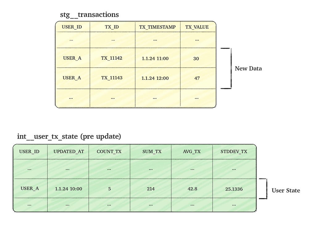
Consider a transactions table named stg__transactions, which tracks user transactions (events). Our goal is to create a time-static table, int__user_tx_state, that aggregates the ‘state’ of user transactions. The column details for both tables are provided in the picture below.

To make the process efficient, we aim to update the state table incrementally by combining the new incoming transactions data with the existing aggregated data (i.e. the current user state). This approach allows us to calculate the updated user state without scanning through all historical data.

The code below assumes understanding of some dbt concepts, if you’re unfamiliar with it, you may still be able to understand the code, although I strongly encourage going through dbt’s incremental guide or read this awesome post.

We’ll construct a full dbt SQL step by step, aiming to calculate incremental aggregations efficiently without repeatedly scanning the entire table. The process begins by defining the model as incremental in dbt and using unique_key to update existing rows rather than inserting new ones.

-- depends_on: {{ ref('stg__transactions') }}
{{ config(materialized='incremental', unique_key=['USER_ID'], incremental_strategy='merge') }}

Next, we fetch records from the stg__transactions table.
The is_incremental block filters transactions with timestamps later than the latest user update, effectively including “only new transactions”.

WITH NEW_USER_TX_DATA AS (
    SELECT
        USER_ID,
        TX_ID,
        TX_TIMESTAMP,
        TX_VALUE
    FROM {{ ref('stg__transactions') }}
    {% if is_incremental() %}
      WHERE TX_TIMESTAMP > COALESCE((select max(UPDATED_AT) from {{ this }}), 0::TIMESTAMP_NTZ)
    {% endif %}
)

After retrieving the new transaction records, we aggregate them by user, allowing us to incrementally update each user’s state in the following CTEs.

INCREMENTAL_USER_TX_DATA AS (
    SELECT
        USER_ID,
        MAX(TX_TIMESTAMP) AS UPDATED_AT,
        COUNT(TX_VALUE) AS INCREMENTAL_COUNT,
        AVG(TX_VALUE) AS INCREMENTAL_AVG,
        SUM(TX_VALUE) AS INCREMENTAL_SUM,
        COALESCE(STDDEV(TX_VALUE), 0) AS INCREMENTAL_STDDEV,
    FROM
        NEW_USER_TX_DATA
    GROUP BY
        USER_ID
)

Now we get to the heavy part where we need to actually calculate the aggregations. When we’re not in incremental mode (i.e. we don’t have any “state” rows yet) we simply select the new aggregations

NEW_USER_CULMULATIVE_DATA AS (
    SELECT
        NEW_DATA.USER_ID,
        {% if not is_incremental() %}
            NEW_DATA.UPDATED_AT AS UPDATED_AT,
            NEW_DATA.INCREMENTAL_COUNT AS COUNT_TX,
            NEW_DATA.INCREMENTAL_AVG AS AVG_TX,
            NEW_DATA.INCREMENTAL_SUM AS SUM_TX,
            NEW_DATA.INCREMENTAL_STDDEV AS STDDEV_TX
        {% else %}
        ...

But when we’re in incremental mode, we need to join past data and combine it with the new data we created in the INCREMENTAL_USER_TX_DATA CTE based on the formula described above.
We start by calculating the new SUM, COUNT and AVG:

  ...
  {% else %}
      COALESCE(EXISTING_USER_DATA.COUNT_TX, 0) AS _n, -- this is n
      NEW_DATA.INCREMENTAL_COUNT AS _k,  -- this is k
      COALESCE(EXISTING_USER_DATA.SUM_TX, 0) + NEW_DATA.INCREMENTAL_SUM AS NEW_SUM_TX,  -- new sum
      COALESCE(EXISTING_USER_DATA.COUNT_TX, 0) + NEW_DATA.INCREMENTAL_COUNT AS NEW_COUNT_TX,  -- new count
      NEW_SUM_TX / NEW_COUNT_TX AS AVG_TX,  -- new avg
   ...

We then calculate the variance formula’s three parts

1. The existing weighted variance, which is truncated to 0 if the previous set is composed of one or less items:

    ...
      CASE
          WHEN _n > 1 THEN (((_n - 1) / (NEW_COUNT_TX - 1)) * POWER(COALESCE(EXISTING_USER_DATA.STDDEV_TX, 0), 2))
          ELSE 0
      END AS EXISTING_WEIGHTED_VARIANCE,  -- existing weighted variance
    ...

2. The incremental weighted variance in the same way:

    ...
      CASE
          WHEN _k > 1 THEN (((_k - 1) / (NEW_COUNT_TX - 1)) * POWER(NEW_DATA.INCREMENTAL_STDDEV, 2))
          ELSE 0
      END AS INCREMENTAL_WEIGHTED_VARIANCE,  -- incremental weighted variance
    ...

3. The mean difference variance, as outlined earlier, along with SQL join terms to include past data.

    ...
      POWER((COALESCE(EXISTING_USER_DATA.AVG_TX, 0) - NEW_DATA.INCREMENTAL_AVG), 2) AS MEAN_DIFF_SQUARED,
      CASE
          WHEN NEW_COUNT_TX = 1 THEN 0
          ELSE (_n * _k) / (NEW_COUNT_TX * (NEW_COUNT_TX - 1))
      END AS BETWEEN_GROUP_WEIGHT,  -- between group weight
      BETWEEN_GROUP_WEIGHT * MEAN_DIFF_SQUARED AS MEAN_DIFF_VARIANCE,  -- mean diff variance
      EXISTING_WEIGHTED_VARIANCE + INCREMENTAL_WEIGHTED_VARIANCE + MEAN_DIFF_VARIANCE AS VARIANCE_TX,
      CASE
          WHEN _n = 0 THEN NEW_DATA.INCREMENTAL_STDDEV -- no "past" data
          WHEN _k = 0 THEN EXISTING_USER_DATA.STDDEV_TX -- no "new" data
          ELSE SQRT(VARIANCE_TX)  -- stddev (which is the root of variance)
      END AS STDDEV_TX,
      NEW_DATA.UPDATED_AT AS UPDATED_AT,
      NEW_SUM_TX AS SUM_TX,
      NEW_COUNT_TX AS COUNT_TX
  {% endif %}
    FROM
        INCREMENTAL_USER_TX_DATA new_data
    {% if is_incremental() %}
    LEFT JOIN
        {{ this }} EXISTING_USER_DATA
    ON
        NEW_DATA.USER_ID = EXISTING_USER_DATA.USER_ID
    {% endif %}
)

Finally, we select the table’s columns, accounting for both incremental and non-incremental cases:

SELECT
    USER_ID,
    UPDATED_AT,
    COUNT_TX,
    SUM_TX,
    AVG_TX,
    STDDEV_TX
FROM NEW_USER_CULMULATIVE_DATA

By combining all these steps, we arrive at the final SQL model:

-- depends_on: {{ ref('stg__initial_table') }}
{{ config(materialized='incremental', unique_key=['USER_ID'], incremental_strategy='merge') }}
WITH NEW_USER_TX_DATA AS (
    SELECT
        USER_ID,
        TX_ID,
        TX_TIMESTAMP,
        TX_VALUE
    FROM {{ ref('stg__initial_table') }}
    {% if is_incremental() %}
      WHERE TX_TIMESTAMP > COALESCE((select max(UPDATED_AT) from {{ this }}), 0::TIMESTAMP_NTZ)
    {% endif %}
),
INCREMENTAL_USER_TX_DATA AS (
    SELECT
        USER_ID,
        MAX(TX_TIMESTAMP) AS UPDATED_AT,
        COUNT(TX_VALUE) AS INCREMENTAL_COUNT,
        AVG(TX_VALUE) AS INCREMENTAL_AVG,
        SUM(TX_VALUE) AS INCREMENTAL_SUM,
        COALESCE(STDDEV(TX_VALUE), 0) AS INCREMENTAL_STDDEV,
    FROM
        NEW_USER_TX_DATA
    GROUP BY
        USER_ID
),

NEW_USER_CULMULATIVE_DATA AS (
    SELECT
        NEW_DATA.USER_ID,
        {% if not is_incremental() %}
            NEW_DATA.UPDATED_AT AS UPDATED_AT,
            NEW_DATA.INCREMENTAL_COUNT AS COUNT_TX,
            NEW_DATA.INCREMENTAL_AVG AS AVG_TX,
            NEW_DATA.INCREMENTAL_SUM AS SUM_TX,
            NEW_DATA.INCREMENTAL_STDDEV AS STDDEV_TX
        {% else %}
            COALESCE(EXISTING_USER_DATA.COUNT_TX, 0) AS _n, -- this is n
            NEW_DATA.INCREMENTAL_COUNT AS _k,  -- this is k
            COALESCE(EXISTING_USER_DATA.SUM_TX, 0) + NEW_DATA.INCREMENTAL_SUM AS NEW_SUM_TX,  -- new sum
            COALESCE(EXISTING_USER_DATA.COUNT_TX, 0) + NEW_DATA.INCREMENTAL_COUNT AS NEW_COUNT_TX,  -- new count
            NEW_SUM_TX / NEW_COUNT_TX AS AVG_TX,  -- new avg
            CASE
                WHEN _n > 1 THEN (((_n - 1) / (NEW_COUNT_TX - 1)) * POWER(COALESCE(EXISTING_USER_DATA.STDDEV_TX, 0), 2))
                ELSE 0
            END AS EXISTING_WEIGHTED_VARIANCE,  -- existing weighted variance
            CASE
                WHEN _k > 1 THEN (((_k - 1) / (NEW_COUNT_TX - 1)) * POWER(NEW_DATA.INCREMENTAL_STDDEV, 2))
                ELSE 0
            END AS INCREMENTAL_WEIGHTED_VARIANCE,  -- incremental weighted variance
            POWER((COALESCE(EXISTING_USER_DATA.AVG_TX, 0) - NEW_DATA.INCREMENTAL_AVG), 2) AS MEAN_DIFF_SQUARED,
            CASE
                WHEN NEW_COUNT_TX = 1 THEN 0
                ELSE (_n * _k) / (NEW_COUNT_TX * (NEW_COUNT_TX - 1))
            END AS BETWEEN_GROUP_WEIGHT,  -- between group weight
            BETWEEN_GROUP_WEIGHT * MEAN_DIFF_SQUARED AS MEAN_DIFF_VARIANCE,
            EXISTING_WEIGHTED_VARIANCE + INCREMENTAL_WEIGHTED_VARIANCE + MEAN_DIFF_VARIANCE AS VARIANCE_TX,
            CASE
                WHEN _n = 0 THEN NEW_DATA.INCREMENTAL_STDDEV -- no "past" data
                WHEN _k = 0 THEN EXISTING_USER_DATA.STDDEV_TX -- no "new" data
                ELSE SQRT(VARIANCE_TX)  -- stddev (which is the root of variance)
            END AS STDDEV_TX,
            NEW_DATA.UPDATED_AT AS UPDATED_AT,
            NEW_SUM_TX AS SUM_TX,
            NEW_COUNT_TX AS COUNT_TX
        {% endif %}
    FROM
        INCREMENTAL_USER_TX_DATA new_data
    {% if is_incremental() %}
    LEFT JOIN
        {{ this }} EXISTING_USER_DATA
    ON
        NEW_DATA.USER_ID = EXISTING_USER_DATA.USER_ID
    {% endif %}
)

SELECT
    USER_ID,
    UPDATED_AT,
    COUNT_TX,
    SUM_TX,
    AVG_TX,
    STDDEV_TX
FROM NEW_USER_CULMULATIVE_DATA

Throughout this process, we demonstrated how to handle both non-incremental and incremental modes effectively, leveraging mathematical techniques to update metrics like variance and standard deviation efficiently. By combining historical and new data seamlessly, we achieved an optimized, scalable approach for real-time data aggregation.

In this article, we explored the mathematical technique for incrementally calculating standard deviation and how to implement it using dbt’s incremental models. This approach proves to be highly efficient, enabling the processing of large datasets without the need to re-scan the entire dataset. In practice, this leads to faster, more scalable systems that can handle real-time updates efficiently. If you’d like to discuss this further or share your thoughts, feel free to reach out — I’d love to hear your thoughts!

Scaling Statistics: Incremental Standard Deviation in SQL with dbt was originally published in Towards Data Science on Medium, where people are continuing the conversation by highlighting and responding to this story.