Removing Spikes from Raman Spectra with Python: A Step-by-Step Guide

Find, remove and replace spikes with interpolated values

This tutorial is part of a growing series on Data Science for Raman Spectroscopy with Python published in towards data science. It is based on this publication in the journal Analytica Chimica Acta. By following along, you’ll add a valuable tool to your data analysis toolkit — an effective method for cleaning up Raman spectra that’s already used in published research.

Introduction

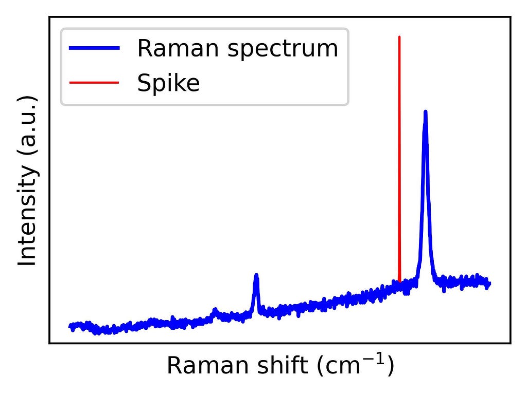
Spike removal is an essential part of Raman data preprocessing. Spikes, caused by cosmic rays impacting the detector, appear as intense, narrow peaks that can distort the analysis. These bursts of energy hit the charge-coupled device (CCD) camera, creating sharp, high-intensity peaks that, if left uncorrected, can interfere with further processing steps like normalization, spectral search, or multivariate data analysis. Cleaning these artifacts is therefore a priority. This tutorial will cover a practical algorithm for removing spikes from Raman spectra. Using Python, we’ll walk through a user-friendly, customizable approach for spike detection and correction to keep Raman data accurate and reliable.

Figure 1 shows an example of a graphene Raman spectrum where a spike is present. Graphene’s exceptional physical properties — such as its electrical and thermal conductivity — have made it a highly studied material. Its Raman spectrum contains peaks that reflect structural characteristics, revealing information about doping, strain, and grain boundaries. Therefore, Raman spectroscopy is a widely used technique to characterize graphene. However, to make the most of this tool, spikes must be previously removed.

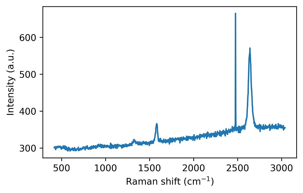
import numpy as np
# Load data directly into a numpy array
data = np.loadtxt(spiked_spectrum.asc, delimiter=',', skiprows=1)

# Extract Raman shift from the first column (index)
ramanshift = data[:, 0]

# Extract intensity from the second column (index 1in Python)
intensity = data[:, 1]

# Plot the data
import matplotlib.pyplot as plt
fig = plt.figure(figsize = (5,3))
plt.plot(ramanshift, intensity)
plt.xlabel('Raman shift (cm$^{-1}$)')
plt.ylabel('Intensity (a.u.)')
plt.show()

The spike removal algorithm

The spike removal algorithm presented here consists of four main steps:

1. Peak finding
2. Spike detection
3. Spike flagging
4. Spectrum correction

Let’s take a look at the different steps with Python code snippets:

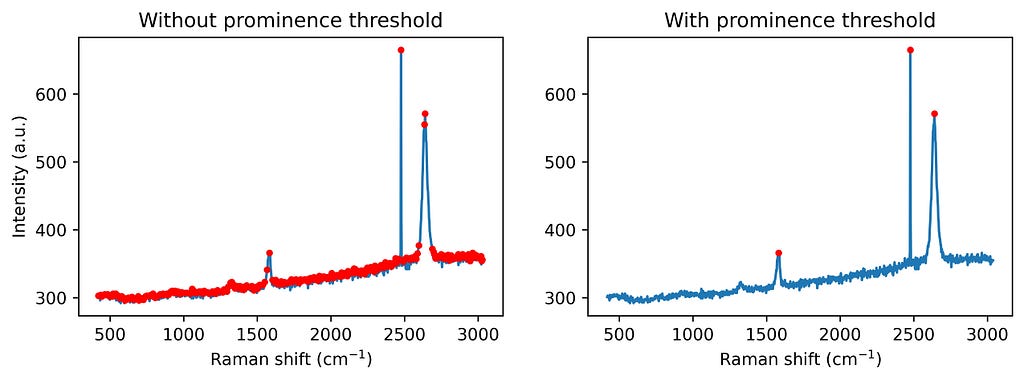
1. Peak finding: First, the algorithm identifies significant peaks by checking for local maxima with a minimum prominence threshold. Adding a prominence threshold helps to exclude small noise-generated peaks, as we don’t aim to correct all the noise. See the following figure for comparison.

from scipy.signal import find_peaks
# Find the peaks in the spectrum (with and without prominence threshold)
peaks_wo_p, _ = find_peaks(intensity) # Peaks found without a prominence threshold
peaks_w_p, _ = find_peaks(intensity, prominence = 20) # Peaks found without a prominence threshold

fig, ax = plt.subplots(1, 2, figsize = (10,3))
ax[0].plot(ramanshift, intensity, zorder=0, label='Raw spectrum')
ax[0].scatter(ramanshift[peaks_wo_p], intensity[peaks_wo_p], marker ='.', color = 'red',label='Found peaks')
ax[1].plot(ramanshift, intensity, zorder=0, label='Raw spectrum')
ax[1].scatter(ramanshift[peaks_w_p], intensity[peaks_w_p], marker ='.', color = 'red',label='Found peaks')
plt.show()

2. Spike detection: Then, spikes are flagged based on their characteristic narrow widths. This point might help in the automation of large spectral datasets. If we know the width of the Raman bands present in our spectra, we can choose a threshold below such a value. For example, with our system resolution, we do not expect to have graphene Raman bands with widths below 10 cm-1.

from scipy.signal import peak_widths
widths = peak_widths(intensity, peaks_w_p)[0]

fig, ax = plt.subplots(figsize = (5,3))
ax.plot(ramanshift, intensity, zorder=0, label='Raw spectrum')
ax2 = ax.twinx()
ax2.scatter(ramanshift[peaks_w_p], widths, marker ='+', color = 'red',label='Peak widths')
plt.show()

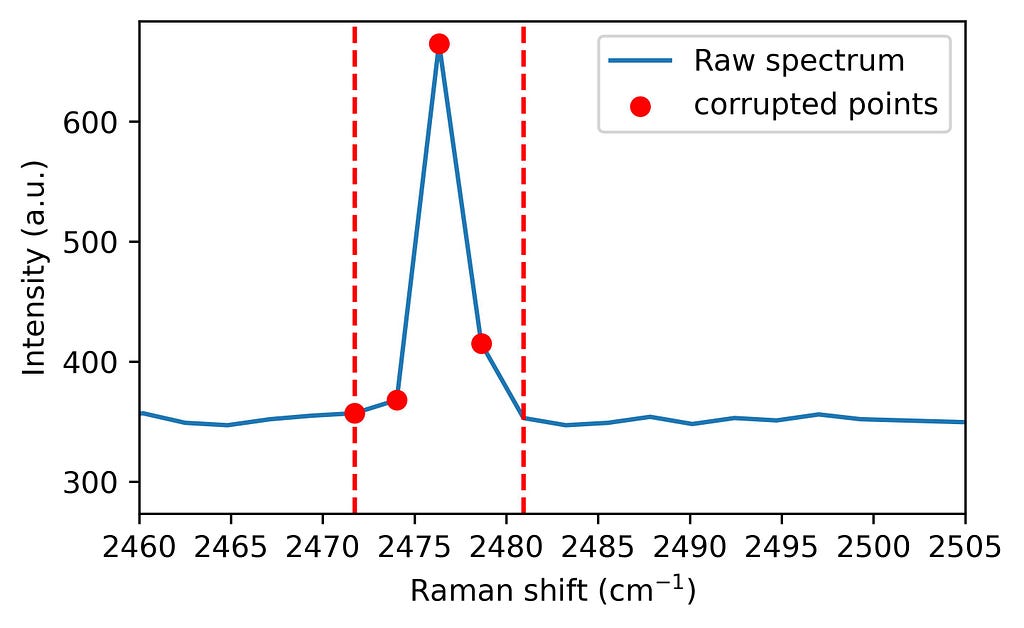
3. Spike flagging Next, any data points affected by spikes are flagged using a range calculated from the peak’s prominence, effectively isolating corrupted pixels. In other words, we select the window that must be corrected

# Let's set the parameters:
width_param_rel = 0.8
width_threshold = 10 # Estimation of the width of the narrowest Raman band

# Calculation of the range where the spectral points are asumed to be corrupted
widths_ext_a = peak_widths(intensity, peaks_w_p, rel_height=width_param_rel)[2]
widths_ext_b = peak_widths(intensity, peaks_w_p, rel_height=width_param_rel)[3]

# Create a vector where spikes will be flag: no spike = 0, spike = 1.
spikes = np.zeros(len(intensity))
    
# Flagging the area previously defined if the peak is considered a spike (width below width_threshold)
for a, width, ext_a, ext_b in zip(range(len(widths)), widths, widths_ext_a, widths_ext_b):
    if width < width_threshold:
        spikes[int(ext_a) - 1: int(ext_b) + 2] = 1 

fig = plt.figure(figsize = (5,3))
plt.plot(ramanshift, intensity, zorder=0,label='Raw spectrum')
a=1
plt.scatter(ramanshift[int(widths_ext_a[a])-1 : int(widths_ext_b[a])+1], 
            intensity[int(widths_ext_a[a])-1 : int(widths_ext_b[a])+1], 
            color ='red', label = 'corrupted points')
plt.axvline(x = ramanshift[int(widths_ext_a[a]) -1], linestyle = '--', color = 'red')
plt.axvline(x = ramanshift[int(widths_ext_b[a]) + 1], linestyle = '--', color = 'red')  
plt.show()

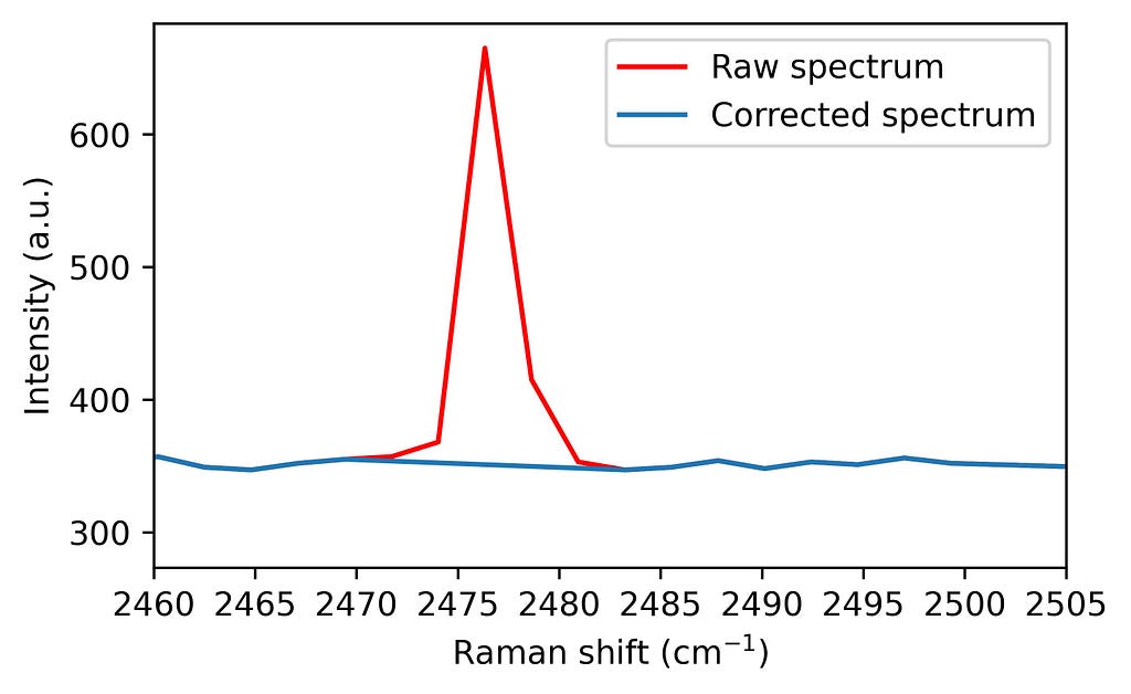
4. Spectrum correction Finally, these points are corrected through interpolation of nearby values, preserving the spectrum’s integrity for subsequent analyses.

from scipy import interpolate
# Let's set the parameter:
moving_average_window = 10

intensity_out = intensity.copy()
    
# Interpolation of corrupted points
for i, spike in enumerate(spikes):
    if spike != 0: # If we have an spike in position i
        window = np.arange(i - moving_average_window, i + moving_average_window + 1) # we select 2 ma + 1 points around our spike
        window_exclude_spikes = window[spikes[window] == 0] # From such interval, we choose the ones which are not spikes
        interpolator = interpolate.interp1d(window_exclude_spikes, intensity[window_exclude_spikes], kind='linear') # We use the not corrupted points around the spike to calculate the interpolation
        intensity_out[i] = interpolator(i) # The corrupted point is exchanged by the interpolated value.

fig = plt.figure(figsize = (5,3))
plt.plot(ramanshift, intensity, zorder=0, color ='red',label='Raw spectrum')
plt.plot(ramanshift, intensity_out, zorder=0, label='Corrected spectrum')
plt.show()

A full spike removal function in Python

All these snippets can be summarized in a single function. This function is designed to be customizable based on your specific data needs, with parameters for adjusting prominence and width:

import numpy as np
from scipy.signal import find_peaks, peak_widths, peak_prominences
from scipy import interpolate

def spike_removal(y, 
                  width_threshold, 
                  prominence_threshold=None, 
                  moving_average_window=10, 
                  width_param_rel=0.8, 
                  interp_type='linear'):
    """
    Detects and replaces spikes in the input spectrum with interpolated values. Algorithm first 
    published by N. Coca-Lopez in Analytica Chimica Acta. https://doi.org/10.1016/j.aca.2024.342312

    Parameters:
    y (numpy.ndarray): Input spectrum intensity.
    width_threshold (float): Threshold for peak width.
    prominence_threshold (float): Threshold for peak prominence.
    moving_average_window (int): Number of points in moving average window.
    width_param_rel (float): Relative height parameter for peak width.
    tipo: type of interpolation (linear, quadratic, cubic)
    
    Returns:
    numpy.ndarray: Signal with spikes replaced by interpolated values.
    """

    # First, we find all peaks showing a prominence above prominence_threshold on the spectra
    peaks, _ = find_peaks(y, prominence=prominence_threshold)
    
    # Create a vector where spikes will be flag: no spike = 0, spike = 1.
    spikes = np.zeros(len(y))
    
    # Calculation of the widths of the found peaks
    widths = peak_widths(y, peaks)[0]
    
    # Calculation of the range where the spectral points are asumed to be corrupted
    widths_ext_a = peak_widths(y, peaks, rel_height=width_param_rel)[2]
    widths_ext_b = peak_widths(y, peaks, rel_height=width_param_rel)[3]
    
    # Flagging the area previously defined if the peak is considered a spike (width below width_threshold)
    for a, width, ext_a, ext_b in zip(range(len(widths)), widths, widths_ext_a, widths_ext_b):
        if width < width_threshold:
            spikes[int(ext_a) - 1: int(ext_b) + 2] = 1 
            
    y_out = y.copy()
    
    # Interpolation of corrupted points
    for i, spike in enumerate(spikes):
        if spike != 0: # If we have an spike in position i
            window = np.arange(i - moving_average_window, i + moving_average_window + 1) # we select 2 ma + 1 points around our spike
            window_exclude_spikes = window[spikes[window] == 0] # From such interval, we choose the ones which are not spikes
            interpolator = interpolate.interp1d(window_exclude_spikes, y[window_exclude_spikes], kind=interp_type) # We use the not corrupted points around the spike to calculate the interpolation
            y_out[i] = interpolator(i) # The corrupted point is exchanged by the interpolated value.
            
    return y_out

The function with the algorithm can then be applied to the spiked graphene spectrum as follows:

intensity_despiked = spike_removal(intensity, 
                                     width_threshold = 3, 
                                     prominence_threshold = 20, 
                                     moving_average_window=10, 
                                     width_param_rel=0.8, 
                                     interp_type='linear')

fig, ax = plt.subplots(1, 2, figsize = (2*5,3))
ax[0].plot(ramanshift, intensity, label = 'spike', color ='red', linewidth = 0.9)
ax[0].plot(ramanshift, intensity_despiked)
ax[1].plot(ramanshift, intensity_despiked)
plt.show()

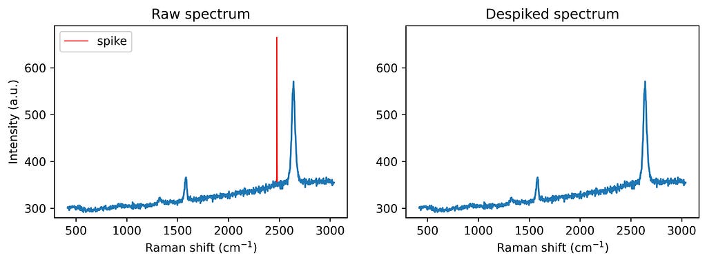
With this spike removal approach, you can ensure your Raman spectra are clean and reliable, minimizing artefacts without losing essential spectral details. The method is ideal for automation, especially if the expected minimum peak width is known, making it highly adaptable for large-scale spectral datasets and high-throughput analysis

I hope you enjoyed this tutorial. Feel free to drop any questions or share your own Raman data challenges in the comments — I’d love to hear how this algorithm helps in your projects!

Ready to try it out? Download the Jupyter Notebook here. And if you found this useful, please, remember to cite the original work, that would help me a lot! 🙂

Removing Spikes from Raman Spectra with Python: A Step-by-Step Guide was originally published in Towards Data Science on Medium, where people are continuing the conversation by highlighting and responding to this story.