Understanding AI applications in bio for machine learning engineers

Anyone who has tried teaching a dog new tricks knows the basics of reinforcement learning. We can modify the dog’s behavior by repeatedly offering rewards for obedience and punishments for misbehavior. In reinforcement learning (RL), the dog would be an agent, exploring its environment and receiving rewards or penalties based on the available actions. This very simple concept has been formalized mathematically and extended to advance the fields of self-driving and self-driving/autonomous labs.
As a New Yorker, who finds herself riddled with anxiety driving, the benefits of having a stoic robot chauffeur are obvious. The benefits of an autonomous lab only became apparent when I considered the immense power of the new wave of generative AI biology tools. We can generate a huge volume of high-quality hypotheses and are now bottlenecked by experimental validation.
If we can utilize reinforcement learning (RL) to teach a car to drive itself, can we also use it to churn through experimental validations of AI-generated ideas? This article will continue our series, Understanding AI Applications in Bio for ML Engineers, by learning how reinforcement learning is applied in self-driving cars and autonomous labs (for example, AlphaFlow).
Self-Driving Cars
The most general way to think about RL is that it’s a learning method by doing. The agent interacts with its environment, learns what actions produce the highest rewards, and avoids penalties through trial and error. If learning through trial and error going 65mph in a 2-ton metal box sounds a bit terrifying, and like something that a regulator would not approve of, you’d be correct. Most RL driving has been done in simulation environments, and current self-driving technology still focuses on supervised learning techniques. But Alex Kendall proved that a car could teach itself to drive with a couple of cheap cameras, a massive neural network, and twenty minutes. So how did he do it?
More mainstream self driving approaches use specialized modules for each of subproblem: vehicle management, perception, mapping, decision making, etc. But Kendalls’s team used a deep reinforcement learning approach, which is an end-to-end learning approach. This means, instead of breaking the problem into many subproblems and training algorithms for each one, one algorithm makes all the decisions based on the input (input-> output). This is proposed as an improvement on supervised approaches because knitting together many different algorithms results in complex interdependencies.
Reinforcement learning is a class of algorithms intended to solve Markov Decision Problem (MDP), or decision-making problem where the outcomes are partially random and partially controllable. Kendalls’s team’s goal was to define driving as an MDP, specifically with the simplified goal of lane-following. Here is a breakdown of how how reinforcement learning components are mapped to the self-driving problem:
- The agent A, which is the decision maker. This is the driver.
- The environment, which is everything the agent interacts with. e.g. the car and its surrounding.
- The state S, a representation of the current situation of the agent. Where the car is on the road. Many sensors could be used determine state, but in Kendall’s example, only a monocular camera image was used. In this way, it’s much closer to what information a human has when driving. The image is then represented in the model using a Variational Autoencoder (VAE).
- The action A, a choice the agent makes that affects the environment. Where and how to brake, turn, or accelerate.
- The reward, feedback from the environment on the previous action. Kendall’s team selected “the distance travelled by the vehicle without the safety driver taking control” as the reward.
- The policy, a strategy the agent uses to decide which action to take in a given state. In deep reinforcement learning, the policy is governed by a deep neural network, in this case a deep deterministic policy gradients (DDPG). This is an off-the-shelf reinforcement learning algorithm with no task-specific adaptation. It is also known as the actor network.
- The value function, the estimator of the expected reward the agent can achieve from a given state (or state-action pair). Also known as a critic network. The critic helps guide the actor by providing feedback on the quality of actions during training.
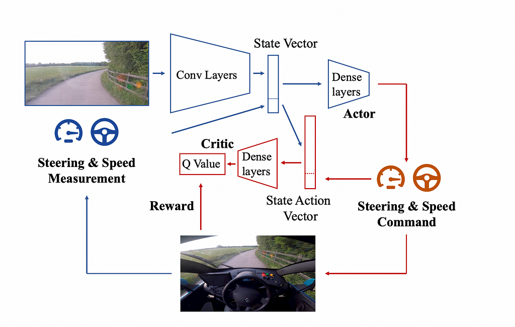
These pieces come together through an iterative learning process. The agent uses its policy to take actions in the environment, observes the resulting state and reward, and updates both the policy (via the actor) and the value function (via the critic). Here’s how it works step-by-step:
- Initialization: The agent starts with a randomly initialized policy (actor network) and value function (critic network). It has no prior knowledge of how to drive.
- Exploration: The agent explores the environment by taking actions that include some randomness (exploration noise). This ensures the agent tries a wide range of actions to learn their effects, while terrifying regulators.
- State Transition: Based on the agent’s action, the environment responds, providing a new state (e.g., the next camera image, speed, and steering angle) and a reward (e.g., the distance traveled without intervention or driving infraction).
- Reward Evaluation: The agent evaluates the quality of its action by observing the reward. Positive rewards encourage desirable behaviors (like staying in the lane), while sparse or no rewards prompt improvement.
- Learning Update: The agent uses the reward and the observed state transition to update its neural networks:
- Critic Network (Value Function): The critic updates its estimate of the Q-function (the function which estimates the reward given an action and state), minimizing the temporal difference (TD) error to improve its prediction of long-term rewards.
- Actor Network (Policy): The actor updates its policy by using feedback from the critic, gradually favoring actions that the critic predicts will yield higher rewards.
6. Replay Buffer: Experiences (state, action, reward, next state) are stored in a replay buffer. During training, the agent samples from this buffer to update its networks, ensuring efficient use of data and stability in training.
7. Iteration: The process repeats over and over. The agent refines its policy and value function through trial and error, gradually improving its driving ability.
8. Evaluation: The agent’s policy is tested without exploration noise to evaluate its performance. In Kendall’s work, this meant assessing the car’s ability to stay in the lane and maximize the distance traveled autonomously.
Getting in a car and driving with randomly initialized weights seems a bit daunting! Luckily, what Kendall’s team realized hyper-parameters can be tuned in 3D simulations before being transferred to the real world. They built a simulation engine in Unreal Engine 4 and then ran a generative model for country roads, varied weather conditions and road textures to create training simulations. This vital tuned reinforcement learning parameters like learning rates, number of gradient steps. It also confirmed that a continuous action space was preferable to a discrete one and that DDPG was an appropriate algorithm for the problem.
One of the most interesting aspects of this was how generalized it is versus the mainstream approach. The algorithms and sensors employed are much less specialized than those required by the approaches from companies like Cruise and Waymo. It doesn’t require advancing mapping data or LIDAR data which could make it scalable to new roads and unmapped rural areas.
On the other hand, some downsides of this approach are:
- Sparse Rewards. We don’t often fail to stay in the lane, which means the reward only comes from staying in the lane for a long time.
- Delayed Rewards. Imagine getting on the George Washington Bridge, you need to pick a lane long before you get on the bridge. This delays the reward making it harder for the model to associate actions and rewards.
- High Dimensionality. Both the state space and available actions have a number of dimensions. With more dimensions, the RL model is prone to overfitting or instability due to the sheer complexity of the data.
That being said, Kendall’s team’s achievement is an encouraging step towards autonomous driving. Their goal of lane following was intentionally simplified and illustrates the ease at with RL could be incorperated to help solve the self driving problem. Now lets turn to how it can be applied in labs.
Self-Driving Labs (SDLs)
The creators of AlphaFlow argue that much like Kendall’s assessment of driving, that development of lab procotols are a Markov Decision Problem. While Kendall constrained the problem to lane-following, the AlphaFlow team constrained their SDL problem to the optimization of multi-step chemical processes for shell-growth of core-shell semiconductor nanoparticles. Semiconductor nanoparticles have a wide range of applications in solar energy, biomedical devices, fuel cells, environmental remediation, batteries, etc. Methods for discovering types of these materials are typically time-consuming, labor-intensive, and resource-intensive and subject to the curse of dimensionality, the exponential increase in a parameter space size as the dimensionality of a problem increases.
Their RL based approach, AlphaFlow, successfully identified and optimized a novel multi-step reaction route, with up to 40 parameters, that outperformed conventional sequences. This demonstrates how closed-loop RL based approaches can accelerate fundamental knowledge.
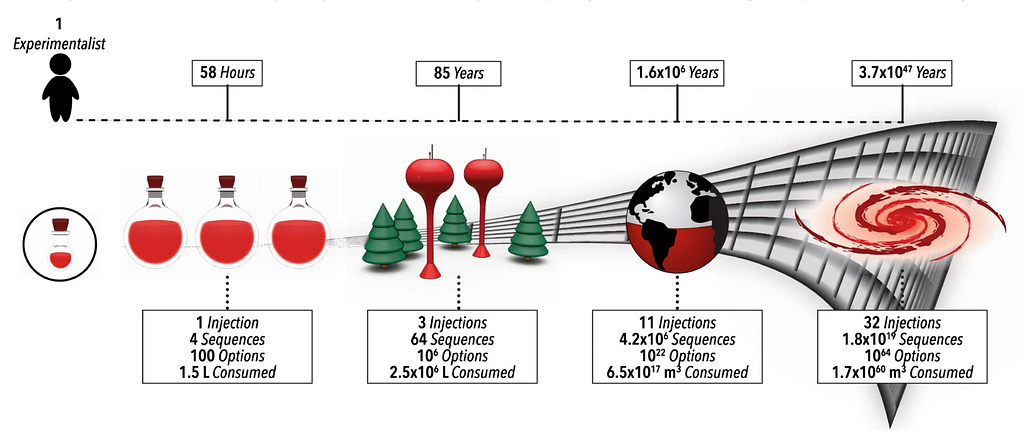
Colloidal atomic layer deposition (cALD) is a technique used to create core-shell nanoparticles. The material is grown in a layer-by-layer manner on colloidal particles or quantum dots. The process involves alternating reactant addition steps, where a single atomic or molecular layer is deposited in each step, followed by washing to remove excess reagents. The outcomes of steps can vary due to hidden states or intermediate conditions. This variability reinforces the belief that this as a Markov Decision Problem.
Additionally, the layer-by-layer manner aspect of the technique makes it well suited to an RL approach where we need clear definitions of the state, available actions, and rewards. Furthermore, the reactions are designed to naturally stop after forming a single, complete atomic or molecular layer. This means the experiment is highly controllable and suitable for tools like micro-droplet flow reactors.
Here is how the components of reinforcement learning are mapped to the self driving lab problem:
- The agent A decides the next chemical step (either a new surface reaction, ligand addition, or wash step)
- The environment is a high-efficiency micro-droplet flow reactor that autonomously conducts experiments.
- The state S represents the current setup of reagents, reaction parameters, and short-term memory (STM). In this example, the STM consists of the four prior injection conditions.
- The actions A are choices like reagent addition, reaction timing, and washing steps.
- The reward is the in situ optically measured characteristics of the product.
- The policy and value function are the RL algorithm which predicts the expected reward and optimizes future decisions. In this case, a belief network composed of an ensemble neural network regressor (ENN) and a gradient-boosted decision tree that classifies the state-action pairs as either viable or unviable.
- The rollout policy uses the belief model to predict the outcome/reward of hypothetical future action sequences and decides the next best action to take using a decision policy applied across all predicted action sequences.
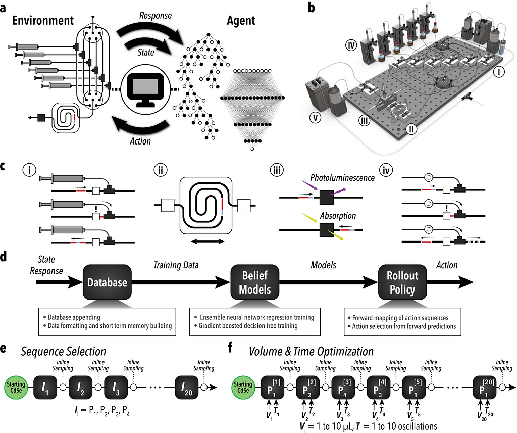
(a) RL-based feedback loop between the learning agent and the automated experimental setup.
(b) Schematic of the reactor system with key modules: reagent injection, droplet mixing, optical sampling, phase separation, waste collection, and refill.
(c ) Breakdown of core module functions: formulation, synthesis, characterization, and phase separation.
(d) Flow diagram showing how the learning agent selects conditions.
(e, f) Overview of reaction space exploration and optimization: sequence selection of reagent injections (P1: oleylamine, P2: sodium sulfide, P3: cadmium acetate, P4: formamide) and volume-time optimization based on the learned sequence.
Similar to the usage of the Unreal Engine by Kendall’s team, the AlphaFlow team used a digital twin structure to help pre-train hyper-parameters before conducting physical experiments. This allowed the model to learn through simulated computational experiments and explore in a more cost efficient manner.
Their approach successfully explored and optimized a 40-dimensional parameter space showcasing how RL can be used to solve complex, multi-step reactions. This advancement could be critical for increasing the throughput experimental validation and helping us unlock advances in a range of fields.
Conclusion
In this post, we explored how reinforcement learning can be applied for self driving and automating lab work. While there are challenges, applications in both domains show how RL can be useful for automation. The idea of furthering fundamental knowledge through RL is of particular interest to the author. I look forward to learning more about emerging applications of reinforcement learning in self driving labs.
Cheers and thank you for reading this edition of Understanding AI Applications in Bio for ML Engineers
Reinforcement Learning: Self-Driving Cars to Self-Driving Labs was originally published in Towards Data Science on Medium, where people are continuing the conversation by highlighting and responding to this story.
Originally appeared here:
Reinforcement Learning: Self-Driving Cars to Self-Driving Labs
Go Here to Read this Fast! Reinforcement Learning: Self-Driving Cars to Self-Driving Labs
