Scaling reinforcement learning from tabular methods to large spaces

Reinforcement learning is a domain in machine learning that introduces the concept of an agent learning optimal strategies in complex environments. The agent learns from its actions, which result in rewards, based on the environment’s state. Reinforcement learning is a challenging topic and differs significantly from other areas of machine learning.
What is remarkable about reinforcement learning is that the same algorithms can be used to enable the agent adapt to completely different, unknown, and complex conditions.
Note. To fully understand the concepts included in this article, it is highly recommended to be familiar with concepts discussed in previous articles.
About this article
Up until now, we have only been discussing tabular reinforcement learning methods. In this context, the word “tabular” indicates that all possible actions and states can be listed. Therefore, the value function V or Q is represented in the form of a table, while the ultimate goal of our algorithms was to find that value function and use it to derive an optimal policy.
However, there are two major problems regarding tabular methods that we need to address. We will first look at them and then introduce a novel approach to overcome these obstacles.
This article is based on Chapter 9 of the book “Reinforcement Learning” written by Richard S. Sutton and Andrew G. Barto. I highly appreciate the efforts of the authors who contributed to the publication of this book.
1. Computation
The first aspect that has to be clear is that tabular methods are only applicable to problems with a small number of states and actions. Let us recall a blackjack example where we applied the Monte Carlo method in part 3. Despite the fact that there were only 200 states and 2 actions, we got good approximations only after executing several million episodes!
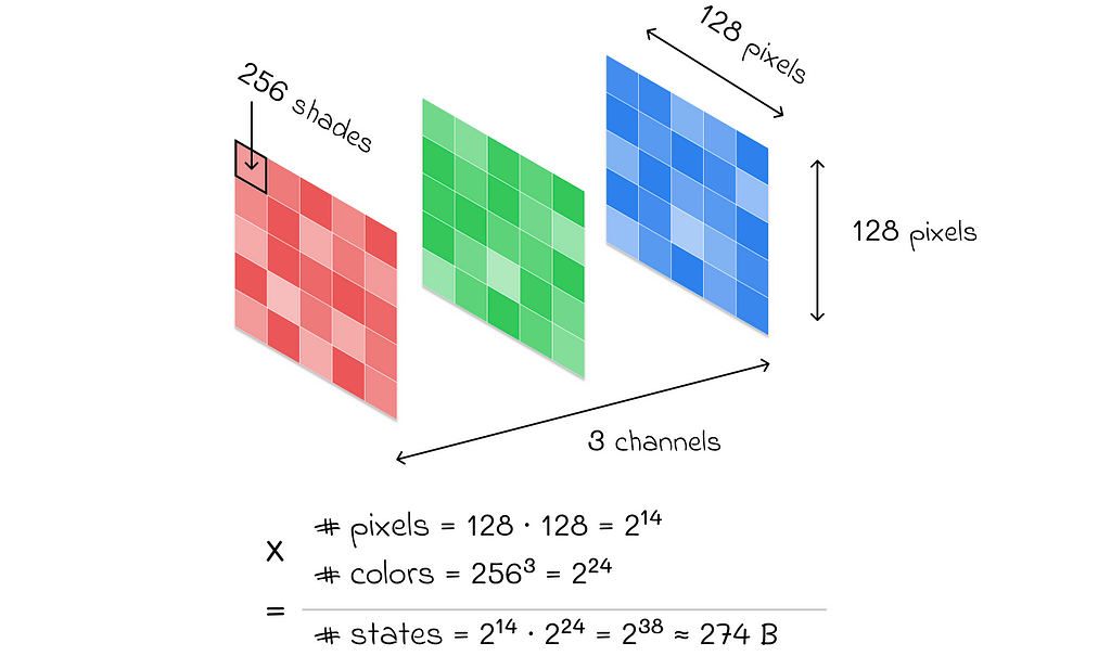
Imagine what colossal computations we would need to perform if we had a more complex problem. For example, if we were dealing with RGB images of size 128 × 128, then the total number of states would be 3 ⋅ 256 ⋅ 256 ⋅ 128 ⋅ 128 ≈ 274 billion. Even with modern technological advancements, it would be absolutely impossible to perform the necessary computations to find the value function!

In reality, most environments in reinforcement learning problems have a huge number of states and possible actions that can be taken. Consequently, value function estimation with tabular methods is no longer applicable.
2. Generalization
Even if we imagine that there are no problems regarding computations, we are still likely to encounter states that are never visited by the agent. How can standard tabular methods evaluate v- or q-values for such states?

This article will propose a novel approach based on supervised learning that will efficiently approximate value functions regardless the number of states and actions.
Idea
The idea of value-function approximation lies in using a parameterized vector w that can approximate a value function. Therefore, from now on, we will write the value function v̂ as a function of two arguments: state s and vector w:

Our objective is to find v̂ and w. The function v̂ can take various forms but the most common approach is to use a supervised learning algorithm. As it turns out, v̂ can be a linear regression, decision tree, or even a neural network. At the same time, any state s can be represented as a set of features describing this state. These features serve as an input for the algorithm v̂.
Why are supervised learning algorithms used for v̂?
It is known that supervised learning algorithms are very good at generalization. In other words, if a subset (X₁, y₁) of a given dataset D for training, then the model is expected to also perform well for unseen examples X₂.
At the same time, we highlighted above the generalization problem for reinforcement learning algorithms. In this scenario, if we apply a supervised learning algorithm, then we should no longer worry about generalization: even if a model has not seen a state, it would still try to generate a good approximate value for it using available features of the state.
Example
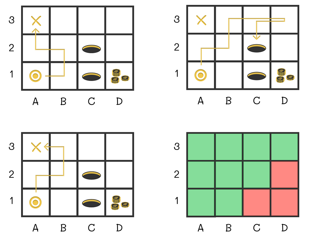
Let us return to the maze and show an example of how the value function can look. We will represent the current state of the agent by a vector consisting of two components:
- x₁(s) is the distance between the agent and the terminal state;
- x₂(s) is the number of traps located around the agent.
For v, we can use the scalar product of s and w. Assuming that the agent is currently located at cell B1, the value function v̂ will take the form shown in the image below:

Difficulties
With the presented idea of supervised learning, there are two principal difficulties we have to address:
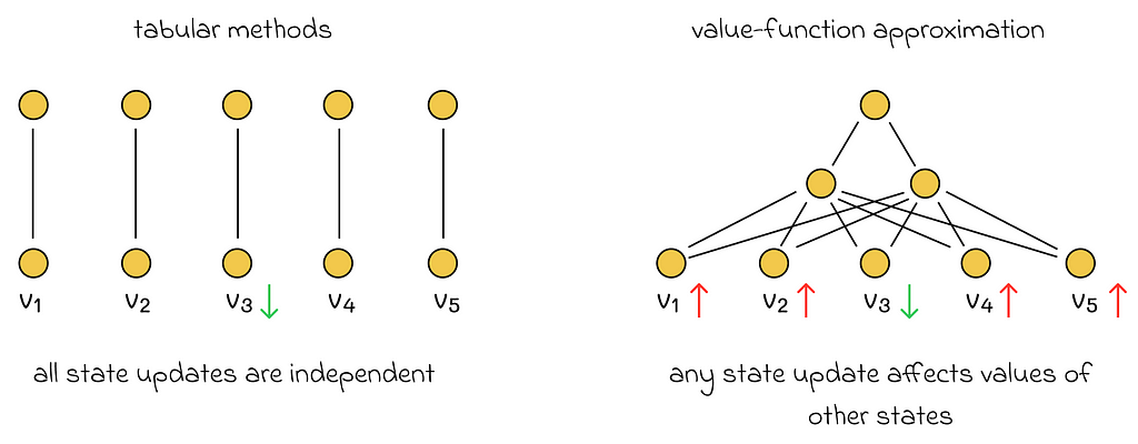
1. Learned state values are no longer decoupled. In all previous algorithms we discussed, an update of a single state did not affect any other states. However, now state values depend on vector w. If the vector w is updated during the learning process, then it will change the values of all other states. Therefore, if w is adjusted to improve the estimate of the current state, then it is likely that estimations of other states will become worse.

2. Supervised learning algorithms require targets for training that are not available. We want a supervised algorithm to learn the mapping between states and true value functions. The problem is that we do not have any true state values. In this case, it is not even clear how to calculate a loss function.
The prediction objective
State distribution
We cannot completely get rid of the first problem, but what we can do is to specify how much each state is important to us. This can be done by creating a state distribution that maps every state to its importance weight.
This information can then be taken into account in the loss function.
Most of the time, μ(s) is chosen proportionally to how often state s is visited by the agent.
Loss function
Assuming that v̂(s, w) is differentiable, we are free to choose any loss function we like. Throughout this article, we will be looking at the example of the MSE (mean squared error). Apart from that, to account for the state distribution μ(s), every error term is scaled by its corresponding weight:

In the shown formula, we do not know the true state values v(s). Nevertheless, we will be able to overcome this issue in the next section.
Objective
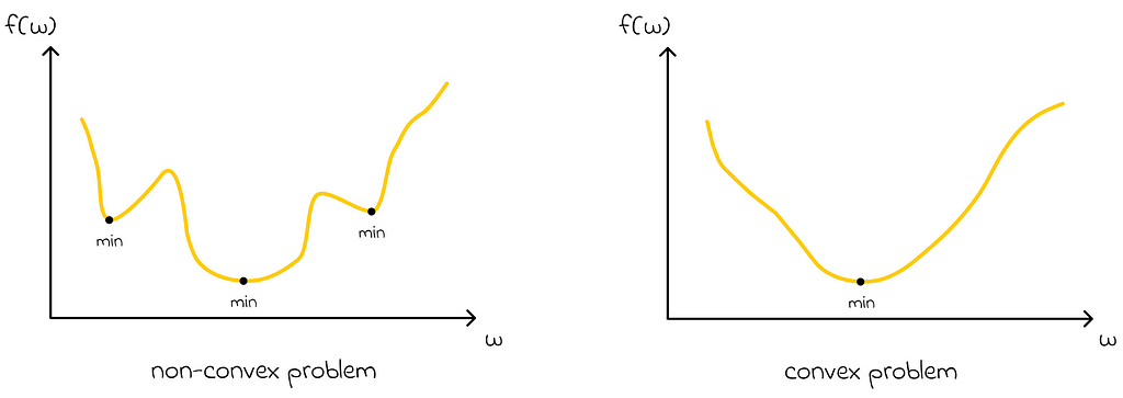
After having defined the loss function, our ultimate goal becomes to find the best vector w that will minimize the objective VE(w). Ideally, we would like to converge to the global optimum, but in reality, the most complex algorithms can guarantee convergence only to a local optimum. In other words, they can find the best vector w* only in some neighbourhood of w.

Despite this fact, in many practical cases, convergence to a local optimum is often enough.
Stochastic-gradient methods
Stochastic-gradient methods are among the most popular methods to perform function approximation in reinforcement learning.
Let us assume that on iteration t, we run the algorithm through a single state example. If we denote by wₜ a weight vector at step t, then using the MSE loss function defined above, we can derive the update rule:

We know how to update the weight vector w but what can we use as a target in the formula above? First of all, we will change the notation a little bit. Since we cannot obtain exact true values, instead of v(S), we are going to use another letter U, which will indicate that true state values are approximated.

The ways the state values can be approximated are discussed in the following sections.
Gradient Monte Carlo
Monte Carlo is the simplest method that can be used to approximate true values. What makes it great is that the state values computed by Monte Carlo are unbiased! In other words, if we run the Monte Carlo algorithm for a given environment an infinite number of times, then the averaged computed state values will converge to the true state values:

Why do we care about unbiased estimations? According to theory, if target values are unbiased, then SGD is guaranteed to converge to a local optimum (under appropriate learning rate conditions).
In this way, we can derive the Gradient Monte Carlo algorithm, which uses expected returns Gₜ as values for Uₜ:

Once the whole episode is generated, all expected returns are computed for every state included in the episode. The respective expected returns are used during the weight vector w update. For the next episode, new expected returns will be calculated and used for the update.
As in the original Monte Carlo method, to perform an update, we have to wait until the end of the episode, and that can be a problem in some situations. To overcome this disadvantage, we have to explore other methods.
Bootstrapping
At first sight, bootstrapping seems like a natural alternative to gradient Monte Carlo. In this version, every target is calculated using the transition reward R and the target value of the next state (or n steps later in the general case):

However, there are still several difficulties that need to be addressed:
- Bootstrapped values are biased. At the beginning of an episode, state values v̂ and weights w are randomly initialized. So it is an obvious fact that on average, the expected value of Uₜ will not approximate true state values. As a consequence, we lose the guarantee of converging to a local optimum.
- Target values depend on the weight vector. This aspect is not typical in supervised learning algorithms and can create complications when performing SGD updates. As a result, we no longer have the opportunity to calculate gradient values that would lead to the loss function minimization, according to the classical SGD theory.
The good news is that both of these problems can be overcome with semi-gradient methods.
Semi-gradient methods
Despite losing important convergence guarantees, it turns out that using bootstrapping under certain constraints on the value function (discussed in the next section) can still lead to good results.

As we have already seen in part 5, compared to Monte Carlo methods, bootstrapping offers faster learning, enabling it to be online and is usually preferred in practice. Logically, these advantages also hold for gradient methods.
Linear methods
Let us look at a particular case where the value function is a scalar product of the weight vector w and the feature vector x(s):

This is the simplest form the value function can take. Furthermore, the gradient of the scalar product is just the feature vector itself:

As a result, the update rule for this case is extremely simple:

The choice of the linear function is particularly attractive because, from the mathematical point of view, value approximation problems become much easier to analyze.
Instead of the SGD algorithm, it is also possible to use the method of least squares.
Linear function in gradient Monte Carlo
The choice of the linear function makes the optimization problem convex. Therefore, there is only one optimum.

In this case, regarding gradient Monte Carlo (if its learning rate α is adjusted appropriately), an important conclusion can be made:
Since the gradient Monte Carlo method is guaranteed to converge to a local optimum, it is automatically guaranteed that the found local optimum will be global when using the linear value approximation function.
Linear function in semi-gradient methods
According to theory, under the linear value function, gradient one-step TD algorithms also converge. The only subtlety is that the convergence point (which is called the TD fixed point) is usually located near the global optimum. Despite this, the approximation quality with the TD fixed point if often enough in most tasks.
Conclusion
In this article, we have understood the scalability limitations of standard tabular algorithms. This led us to the exploration of value-function approximation methods. They allow us to view the problem from a slightly different angle, which elegantly transforms the reinforcement learning problem into a supervised machine learning task.
The previous knowledge of Monte Carlo and bootstrapping methods helped us elaborate their respective gradient versions. While gradient Monte Carlo comes with stronger theoretical guarantees, bootstrapping (especially the one-step TD algorithm) is still a preferred method due to its faster convergence.
Resources
All images unless otherwise noted are by the author.
Reinforcement Learning, Part 7: Introduction to Value-Function Approximation was originally published in Towards Data Science on Medium, where people are continuing the conversation by highlighting and responding to this story.
Originally appeared here:
Reinforcement Learning, Part 7: Introduction to Value-Function Approximation
