Reinforcement Learning: Introduction and Main Concepts

Making the first step into the world of reinforcement learning

Introduction

Reinforcement learning is a special domain in machine learning that differs a lot from the classic methods used in supervised or unsupervised learning.

The ultimate objective consists of developing a so-called agent that will perform optimal actions in environments. From the start, the agent usually performs very poorly but as time goes on, it adapts its strategy from the trial and error approach by interacting with the environment.

The beauty of reinforcement learning is that the same algorithms can be used to make the agent adapt to absolutely different, unknown, and complex conditions.

Reinforcement learning has a wide range of applications and mostly used when a given problem cannot be solved by classic methods:

• Games. Existing approaches can design optimal game strategies and outperform humans. The most well-known examples are chess and Go.
• Robotics. Advanced algorithms can be incorporated into robots to help them move, carry objects or complete routine tasks at home.
• Autopilot. Reinforcement learning methods can be developed to automatically drive cars, control helicopters or drones.

About this article

Though reinforcement learning is a very exciting and unique area, it is still one of the most sophisticated topics in machine learning. In addition, it is absolutely critical from the beginning to understand all of its basic terminology and concepts.

For these reasons, this article introduces only the key theoretical concepts and ideas that will help the reader to further advance in reinforcement learning.

Additionally, this article is based on the third chapter of the famous book “Reinforcement Learning” written by Richard S. Sutton and Andrew G. Barto, which I would highly recommend to everyone interested in delving deeper.

Apart from that, this book contains practical exercises. Their solutions can be found in this repository.

Reinforcement learning framework

First of all, let us understand the reinforcement learning framework which contains several important terms:

• Agent represents an object whose goal is to learn a strategy to optimize a certain process;
• Environment acts as a world in which the agent is located and consists of a set of different states;
• At each timestamp, the agent can perform an action in the environment that will change the environment’s state to a new one. Additionally, the agent will receive feedback indicating how good or bad the chosen action was. This feedback is called a reward and is represented in the numerical form.
• By using feedback from different states and actions, the agent gradually learns the optimal strategy to maximize the total reward over time.

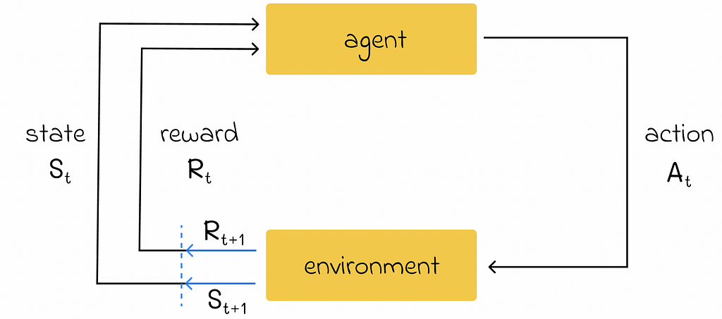
In many cases, given the current state and the agent’s action in that state, the change to a new state can result in different rewards (rather a single one) where each of them corresponds to its own probability.

The formula below considers this fact by summing up over all possible next states and rewards that correspond to them.

To make things more clear, we are going to use the prime ’ symbol to designate a variable in its next step. For example, if s represents the agent’s current state, then s’ will refer to the next agent’s state.

Reward types

To formally define the total reward in the long run, we need to introduce the term the “cumulative reward” (also called “return”) which can take several forms.

Simple formulation

Let us denote Rᵢ as the reward received by the agent at timestamp i, then the cumulative reward can be defined as the sum of rewards received between the next timestamp and the final timestamp T:

Discounted cumulative reward

Most of the time, the discounted cumulative reward is used. It represents the same reward system as before except for the fact that every individual reward in the sum is now multiplied by an exponentially decayed discount coefficient.

The γ (also sometimes denoted as α) parameter in the formula above is called the discount rate and can take a value between 0 and 1. The introduction of discounted reward makes sure that the agent prioritizes actions that result in more short-term rewards. Ultimately, the discounted cumulative reward can be expressed in the recursive form:

Types of tasks

Episodic tasks

In some cases, the interaction between an agent and the environment can include a set of independent episodes. In this scenario, every episode starts independently from others and its beginning state is sampled from the distribution of states.

For instance, imagine that we want the agent to learn the optimal strategy to play a game. To do that, we will run a set of independent games where in each of them a robot can either win or lose. The received rewards in every episode will gradually influence the strategy that the robot will be using in the following games.

Episodes are also referred to as trials.

Continuing tasks

At the same time, not all types of tasks are episodic: some of them can be continuing meaning that they do not have a terminal state. In such cases, it is not always possible to define the cumulative return because the number of timestamps is infinite.

Policies and value functions

Policy

Policy π is a mapping between all possible states s ∈ S to probabilities p of performing any possible action from that state s.

If an agent follows a policy π, then the agent’s probability p(a | s) of performing the action a from state s is equal to p(a | s) = π(s).

By definition, any policy can be represented in the form of a table of size |S| x |A|.

Let us look at the example of the maze game below. The agent that is initially located at the A1 cell. During each step, the agent has to move either horizontally or vertically (not diagonally) to an adjacent cell. The game ends when the agent reaches the terminal state located at C1. The cell A3 contains a large reward that an agent can collect if it steps on it. The cells B1 and C3 are maze walls that cannot be reached.

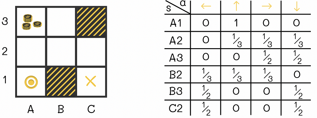
One of the simplest policies that can be used is random: at each state, the agent randomly moves to any allowed cell with equal probability. The corresponding policy for this strategy is illustrated in the figure above.

The demonstrated maze is also an example of an episodic task. After reaching the terminal state and obtaining a certain reward, a new independent game can be initialized.

Apart from policies, in reinforcement learning, it is common to use the notion of value functions which describe how good or bad (in terms of the expected reward) it is for the agent to be in a given state or to take a certain action given the current state.

State-value function

State-value function v(s) (or simply V-function) is a mapping from every environment state to the cumulative expected reward the agent would receive if it were initially placed at that state following a certain policy π.

V-function can be represented as a 1-dimensional table of size |S|.

To better understand the definition of the V-function, let us refer to the previous example. We can see that cells located in the neighbourhood of A3 (which are A2, A3 and B3) have higher V-values than those located further from it (like A1, B2 and C2). This makes sense because being located near a large reward at A3, the agent has a higher chance to collect it.

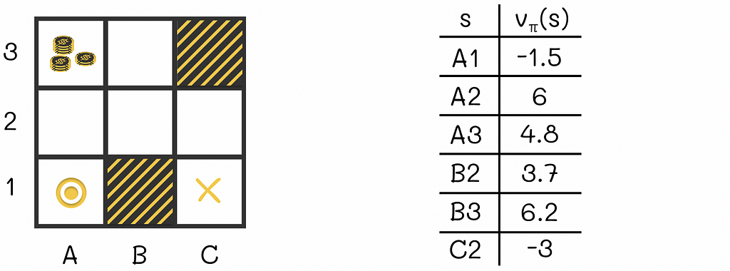
The V-value for terminal states is equal to 0.

Action-value function

Action-value functions have similar concept, in comparison to state-value functions. However, they also take into account a possible action the agent can take under a given policy.

Action-value function q(s, a) (or simply Q-function) is a mapping from each environment state s ∈ S and each possible agent’s action a ∈ A to the expected reward the agent would receive if it were initially placed at that state and had to take that action following a certain policy π.

Q-function can be represented in the form of table of size |S| x |A|.

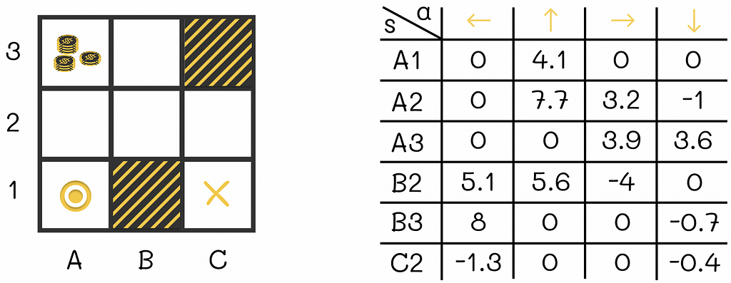
The difference between state and action functions is only in the fact that the action-value function takes additional information about the action the agent is going to take in the current state. The state function only considers the current state and does not take into account the next agent’s action.

Both V- and Q-functions are learned from the agent’s experience.

A subtility on V- and Q-values

Why is q(s, a) ≠ v(s’), i.e. why the expected reward of an agent being in state s and taking the action a leading to next state s’ is not equal to the expected reward of an agent being in state s’?

This question might seem logical at first. Indeed, let us take the agent from the example above who is at cell B2 and assume that it then makes a transition to B3. From the Q-table we can see that the expected reward q(B2, “up”) = 5.6. At the same time, the V-table shows the expected reward v(B3) = 6.2. While 5.6 is relatively close to 6.2, both values are still not equal. So the ultimate question is why q(B2, “up”) ≠ v(B3)?

The answer to this question lies in the fact that despite choosing an action in the current state s that deterministically leads to the next state s’, the reward received by the agent from that transition is taken into account by the Q-function but not by the V-function. In other words, if the current timestamp is t, then the expected reward q(s, a) will consider the discounted sum starting from the step t: Rₜ + αRₜ₊₁ … . The expected reward corresponding to v(s’) will not have the term Rₜ in its sum: Rₜ₊₁ + αRₜ₊₂ + … .

It is worth additionally noting that sometimes an action a taken at some state s can lead to multiple possible next states. The simple maze example above does not demonstrate this concept. But we can add the following condition, for instance, to the agent’s actions: when the agent chooses a direction to move in the maze, there is a 20% chance that the light in the new cell will be turned off and because of that the agent will ultimately move by 90° relatively to that direction.

The introduced concept demonstrates how the same action from the same state can lead to different states. As a consequence, the rewards received by the agent from the same action and state can differ. That is another aspect that contributes to the inequality between q(s, a) and v(s’).

Bellman equation

Bellman equation is one of the fundamental equations in reinforcement learning! In simple words, it recursively establishes the state / action function values at the current and next timestamps.

V-function

By using the definition of the expected value, we can rewrite the expression of the state value function to use the V-function of the next step:

What this equality states is simply the fact that the v-value of the current state s equals the expected value of the sum of the reward received by the agent from transitioning to that state s and the discounted v-value of the next state s’.

In their book, Richard S. Sutton and Andrew G. Barto use so-called “backup diagrams” that allow to better understand the flow of state functions and capture the logic behind the probability multiplication which take places in the Bellman equation. The one used for the V-function is demonstrated below.

Bellman equation plays an important role for computing, approximating and calculating the V-function.

Q-function

Similarly to V-functions, we can derive the Bellman equation for Q-functions.

Optimal policy

Let us define the comparison operation between different policies.

A policy π₁ is said to be better than or equal to policy π₂ if the expected reward of π₁ is greater than or equal to the expected reward of π₂ for all states s ∈ S.

A policy π⁎ is said to be optimal if it is better than or equal to any other policy.

Every optimal policy also has the optimal V⁎- and Q⁎-functions associated with it.

Bellman optimality equation

We can rewrite Bellman equations for optimal policies. In reality, they look very similar to normal Bellman equations we saw before except for the fact that that the policy term π(a|s) is removed and the max function is added to deterministically get the maximum reward from choosing the best action a from the current state s.

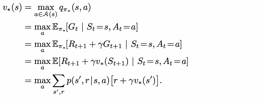
These equations can be mathematically solved for every state. If either the optimal V⁎-function or Q⁎-function is found, the optimal policy π⁎ can also be easily calculated which will always greedily choose the actions that maximise the expected reward.

Unfortunately, it is very hard in practice to mathematically solve Bellman equations because the number of states in most problems is usually huge. For this reason, reinforcement learning methods are used that can approximately calculate optimal policies with much fewer computations and memory requirements.

Conclusion

In this article, we have discussed how agents learn through experience by the trial and error approach. The simplicity of the introduced reinforcement learning framework generalizes well for many problems, yet provides a flexible way to use the notions of policy and value functions. At the same time, the utlimate algorithm objective consists of calculating the optimal V⁎– and Q⁎– functions maximizing the expected reward.

Most of the existing algorithms try to approximate the optimal policy function. While the best solution is almost impossible to get in real-world problems due to memory and computation constraints, approximation methods work very well in most situations.

Resources

• Reinforcement Learning. An Introduction. Second Edition | Richard S. Sutton and Andrew G. Barto
• Reinforcement Learning. Exercise Solutions | GitHub repository (@LyWangPX).

All images unless otherwise noted are by the author.

Reinforcement Learning: Introduction and Main Concepts was originally published in Towards Data Science on Medium, where people are continuing the conversation by highlighting and responding to this story.