Reinforcement Learning for Physical Dynamical Systems: An Alternative Approach

Reintroducing genetic algorithms and comparing to neural networks

Physical and Nonlinear Dynamics

Control theory, through classical, robust, and optimal approaches, enable modern civilization. Refining, telecommunications, modern manufacturing and more depend on them. Control theory has been built on the insight provided by physics equations, such as derived from Newton’s Laws and Maxwell’s equations. These equations describe the dynamics, the interplay of different forces, on physical systems. Through them we understand how the equation moves between states, where a state is “the set of all information that sufficiently describes the system” [1], often in terms of variables such as pressure or velocity of fluid particles in fluid dynamics, or charge and current states in electrodynamics. By deriving equations for the systems, we can predict how the states change through time and space and express this evolution in terms of a differential equation. With this understanding, we can apply controls in the form of specially applied forces to maintain these systems at a desired state or output. Typically, this force is calculated based on the output of the system. Consider a vehicle cruise control. The input is the desired speed, the output the actual speed. The system is the engine. The state estimator observes the speed and determines what the difference between output and input speed is and how apply a control, such as adjusting fuel flow, to reduce the error.

However, for all its accomplishments, control theory encounters substantial limitations. Most control theory is built around linear systems, or systems where a proportional change in input leads to a proportional change in output. While these systems can be quite complex, we have extensive understanding of these systems, affording us practical control of everything from deep ocean submersibles and mining equipment to spacecraft.

However, as Stanislaw Ulam remarked, “using a term like nonlinear science is like referring to the bulk of zoology as the study of non-elephant animals.” Our progress so far in controlling complex physical systems has mostly come through finding ways to limit them to linear behavior. This can cost us efficiency in several ways:

· Break down complex system into component parts that are individually controlled, optimizing for subsystems rather than the system as a whole

· Operate systems at simpler, but less efficient operating modes or not take advantage of complex physics, such as active flow control to reduce aircraft drag

· Tight operating condition limits that can result in unpredictable or catastrophic failure if exceeded

Advanced manufacturing, improved aerodynamics, and complex telecommunications would all benefit from a better approach to control of nonlinear systems.

The fundamental characteristic of nonlinear dynamical systems is their complex response to inputs. Nonlinear systems vary dramatically even with small changes in environment or state. Consider the Navier-Stokes equations that govern fluid flow: the same set of equations describes a placid, slow flowing stream as a raging torrent, and all the eddies and features of the raging torrent are contained within the equation dynamics.

Nonlinear systems present difficulties: unlike linear systems we often don’t have an easily predictable idea of how the system will behave as it transitions from one state to the next. The best we can approach is through general analysis or extensive simulation. Hence, with nonlinear systems we are faced with two problems: system identification — that is, understanding how it will behave at a given state, and system control — how it will change in the short and long term in response to a given input and so what input to make to get the desired outcome.

Reinforcement Learning for Physics

While nonlinear analysis and control continues to make progress, we remain limited in our ability to exploit these systems using traditional, equation-based methods. However, as computing power and sensor technology become more accessible, data-based approaches offer a different approach.

The mass increase in data availability has given rise to machine learning (ML) approaches, and reinforcement learning (RL) provides a new approach to tackling the challenge of controlling nonlinear dynamical systems more effectively. RL, already finding success in environments from self-driving cars to strategy and computer games, is an ML framework which trains algorithms, or agents, “to learn how to make decisions under uncertainty to maximize a long-term benefit through trial and error” [1]. In other words, RL algorithms address the problems of system identification and control optimization and do this not by manipulation and analysis of governing equations, but by sampling the environment to develop a prediction of what input actions lead to desired outcomes. RL algorithms, or agents, apply a policy of actions based on the system state, and refine this policy as they analyze more information on the system.

Many RL algorithms are based on using neural networks to develop functions that map state to optimal behavior. RL problems can be framed as state-action-reward tuples. For a given state, a certain action leads to a given reward. Neural networks act as universal function approximators that can be tuned to accurately approximate the state-action-reward tuple function across an entire system. To do so it must acquire new knowledge by exploring the system or environment, and then refine its policy by exploiting the additional data gained. RL algorithms are differentiated by how they apply mathematics to explore, exploit, band balance between the two.

However, neural networks pose several challenges:

· Resource requirements. Using a neural network to estimate a function that can determine the reward and best action to take for every state can take considerable time and data.

· Explainability. It is often difficult to understand how neural networks are arriving at their solutions, which limits their utility for providing real insight and can make it hard to predict or bound the action of a neural network. Explainability is especially important for physical systems as it would allow the powerful analytical tools developed over several centuries of mathematics to be used to gain additional insight into a system.

While there are approaches, such as transfer learning and topological analysis, to address these challenges, they remain barriers to fuller application of RL. However, an alternate approach may be useful in our case where we are looking specifically at physical systems. Recall that the physical systems we are discussing are defined by, or can be very well described by, mathematical equations. Instead of having to develop a completely arbitrary function, we can focus on trying to find an expression comprised of common mathematical operators: arithmetic, algebraic, and transcendental functions (sine, e^x, etc.). Or means to this end will be using genetic algorithms. As described in [2], genetic algorithms can be adapted to explore function spaces through random generation of functions and exploiting and refining solutions through mutations and cross-breeding of promising candidates.

So, while neural networks are champions of most RL problems, for physical dynamics a new challenger appears. Next we will take a closer look the generic algorithm approach and see how it fairs against a leading RL algorithm, soft actor critic. To do this we will evaluate both in physics-based gymnasiums using AWW Sagemaker Experiments. We will conclude by evaluating the results, discussing conclusions, and suggesting next steps.

Recall that RL faces two challenges, exploring the environment and exploiting the information discovered. Exploration is necessary to find the best policy considering the likelihood of being in any state. Failure to explore means both a global optimum may be missed for a local, and the algorithm may not generalize sufficiently to succeed in all states. Exploitation is needed to refine the current solution to an optimum. However, as an algorithm refines a particular solution, it trades away the ability to explore the system further.

Soft Actor Critic (SAC) is a refinement of the powerful Actor-Critic RL approach. The Actor-Critic family of algorithms approaches the explore/exploit trade off by separating estimation of the state values and associated reward from optimizing a particular policy of inputs. As the algorithm collects new information, it updates each estimator. Actor-Critic has many nuances to its implementation; interested readers should consult books or online tutorials. SAC optimizes the critic by favoring exploration of states which have rewards dramatically different then the critic estimated. OpenAI provides a detailed description of SAC.

For this experiment, we use the Coax implementation of SAC. I looked at several RL libraries, including Coach and Spinning Up, but Coax was one of the few I found to work mostly “out of the box” with current Python builds. The Coax library includes a wide range of RL algorithms, including PPO, TD3, and DDPG and works well with gymnasium.

Actor-critic methods such as SAC are typically implemented through neural networks as the function approximator. As we discussed last time, there is another potential approach to exploring the system and exploiting potential control policies. Genetic algorithms explore through random generation of possible solutions and exploit promising policies by mutating or combining elements (breeding) of different solutions. In this case, we will evaluate a genetic programming variant of genetic algorithms as an alternative means of function approximation; specifically, we will use a genetic approach to randomly generate and then evaluate trees of functions containing constants, state variables, and mathematical functions as potential controllers.

The Genetic Programming (GP) algorithm implemented is adapted from [2] except in place of tournament used by that text, this implementation selects the top 64% (Nn below of 33%) of each generation as eligible for mutation and reseeds the remainder for better exploration of the solution space. To create each individual tree in a generation, a growth function randomly calls from arithmetic functions (+,-,*, /) and transcendental functions (such as e^x, cos (x)) to build branches with constants or state variables as leaves to end branches. Recursive calls are used to build expressions based on Polish notation ([2] implemented via LISP, I have adapted to Python), with rules in place to avoid i.e. divide by 0 and ensure mathematical consistency so that every branch ends correctly in a constant or sensor value leaf. Conceptually, an equation tree appears as:

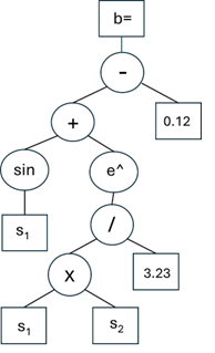
This results in a controller b= sin (s1)+ e^(s1*s2/3.23)-0.12, written by the script as: — + sin s1 e^ / * s1 s2 3.23 0.12, where s denote state variables. It may seem confusing at first but writing out a few examples will clarify the approach.

With a full generation of trees built, each one is then run through the environment to evaluate performance. The trees are then ranked for control performance based on achieved reward. If the desired performance is not met, the best performing tree is preserved, the top 66% are mutated by crossover (swapping elements of two trees), cut and grow (replace an element of a tree), shrink (replace a tree element with a constant) or re-parameterize (replace all constants in a tree) following [2]. This allows exploitation of the most promising solutions. To continue to explore the solution space, the low performing solutions are replaced with random new trees. Each successive generation is then a mix of random new individuals and replications or mutations of the top performing solutions.

Trees are tested against random start locations within the environment. To prevent a “lucky” starting state from skewing results (analogous to overfitting the model), trees are tested against a batch of different random starting states.

Hyperparameters for genetic programming include:

Commented code can be found on github. Note that I am a hobby coder, and my code is kludgy. Hopefully it is at least readable enough to understand my approach, despite any un-pythonic or generally bad coding practice.

Evaluating the Approaches

Both algorithms were evaluated in two different gymnasium environments. The first is the simple pendulum environment provided by gymnasium foundation. The inverted pendulum is a simple nonlinear dynamics problem. The action space is a continuous torque that can be applied to the pendulum. The observation space is the same as the state and is the x,y coordinates and angular velocity. The goal is to hold the pendulum upright. The second is the same gymnasium, but with random noise added to the observation. The noise is normal with mean 0 and variance 0.1 to simulate realistic sensor measurements.

One of the most important parts of RL development is designing a proper reward function. While there are many algorithms that can solve a given RL problem, defining an appropriate reward for those algorithms to optimize to is a key step in making a given algorithm successful for a specific problem. Our reward needs to allow us to compare the results of two different RL approaches while ensuring each proceeds to its goal. Here, for each trajectory we track cumulative reward and average reward. To make this easier, we have each environment run for a fixed number of time steps with a negative reward based on how far from the target state an agent is at each time step. The Pendulum gym operates this way out of the box — truncation at 200 timesteps and a negative reward depending on how far from upright the pendulum is, with a max reward at 0, enforced at every time step. We will use average reward to compare the two approaches.

Our goal is to evaluate convergence speed of each RL framework. We will accomplish this using AWS Sagemaker Experiments, which can automatically track metrics (such as current reward) and parameters (such as active hyperparmeters) across runs by iteration or CPU time. While this monitoring could be accomplished through python tools, Experiments offers streamlined tracking and indexing of run parameters and performance and replication of compute resources. To set up the experiment, I adapted the examples provided by AWS. The SAC and GP algorithms were first assed in local Jupyter notebooks and then uploaded to a git repository. Each algorithm has its own repository and Sagemaker notebook. The run parameters are stored to help classify the run and track performance of different experiment setups. Run metrics, for our cases reward and state vector, are the dependent variables we want to measure to compare the two algorithms. Experiments automatically record CPU time and iteration as independent variables.

Through these experiments we can compare the performance of the champion, a well-developed, mature RL algorithm like SAC, against the contender, a little-known approach coded by a hobby coder without formal RL or python training. This experiment will provide insight into different approaches to developing controllers for complex, non-linear systems. In the next part we will review and discuss results and potential follow-ons.

The first experiment was the default pendulum gymnasium, where the algorithm tries to determine the correct torque to apply to keep pendulum inverted. It ends after a fixed time and gives negative reward based on how far from vertical the pendulum is. Prior to running in Sagemaker experiment, both SAC and GP algorithms were run on my local machine to verify convergence. Running in experiments allowed better tracking of comparable compute time. Results of compute time against average reward per iteration follow:

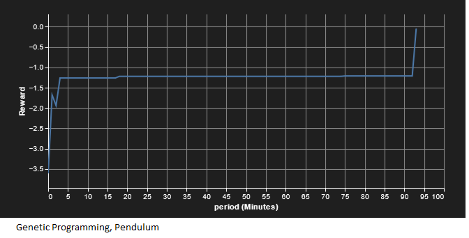
We see that GP, despite being a less mature algorithm, arrived at a solution with far less computational requirement than SAC. On the local run to completion, SAC seemed to take about 400,000 iterations to converge, requiring several hours. The local instantiation was programmed to store recordings of SAC progress throughout training; interestingly SAC seemed to move from learning how to move the pendulum towards the top to learning how to hold the pendulum still, and then combined these, which would explain the dip in the reward as the time when SAC was learning to hold the pendulum steady. With GP we see monotonic increase in reward in steps. This is because the best performing function tree is always retained, so the best reward stays steady until a better controller is calculated.

The second experiment was adding Gaussian noise (0, 0.1) to the state measurement. We see similar results as with the no-noise situation, except with longer convergence times. Results are shown below; again, GP outperforms SAC.

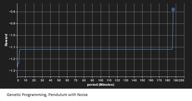
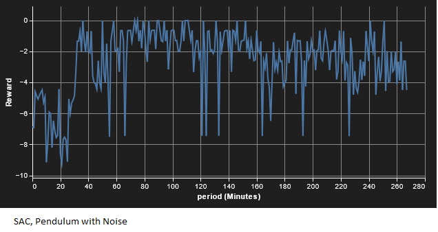
In both cases we see GP perform faster than SAC (as with the previous example, SAC did converge locally, I just didn’t want to pay AWS for the compute time!). However, as many of you have no doubt noticed, this has been a very basic comparison, both in terms of machine learning and physical systems. For example, hyperparameter tunning could result in different results. Still, this is a promising start for the contender algorithm and show it to be worth further investigation.

In the long run, I think GP may offer several benefits over neural network-based approaches like SAC:

· Explainability. While the equation GP finds can be convoluted, it is transparent. Skilled may simplify the equation, helping provide insight into the physics of the determined solution, helpful for determining regions of applicability and increasing trust in the control. Explainability, while an active area of research, remains a challenge for neural networks.

· Informed ML. GP allows easier application of insight into the system under analysis. For example, if the system is known to have sinusoidal behavior, the GP algorithm can be adapted to try more sinusoidal solutions. Alternatively, if a solution is known for a similar or simplified system to the one under study, then that solution can be pre-seeded into the algorithm.

· Stability. With addition of simple safeguards mathematical validity and limit absolute value, GP approaches will remain stable. As long as the top performer is retained each generation then solution will converge, though time bounds on convergence are not guaranteed. Neural network approaches of more common RL do not have such guarantees.

· Developmental Opportunity. GP is relatively immature. The SAC implementation here was one of several available for application, and neural networks have been the benefit of extensive effort to improve performance. GP hasn’t benefit from such optimization; my implementation was built around function rather than efficiency. Despite this, it performed well against SAC, and further improvements from more professional developers could provide high gains in efficiency.

· Parallelizability and modularity. Individual GP equations are simple compared to NNs, the computational cost comes from repeated runs through the environment rathe than environment runs and backpropagation of NNs. It would be easy to split a “forest” of different GP equation trees across different processors to greatly improve computing speed.

However, neural network approaches are used more extensively for good reason:

· Scope. Neural networks are universal function approximators. GP is limited to the terms defined in the function tree. Hence, neural network based approaches can cover a far greater range and complexity of situations. I would not want to try GP to play Starcraft or drive a car.

· Tracking. GP is a refined version of random search, which results, as seen in the experiment, halting improvement.

· Maturity. Because of the extensive work across many different neural based algorithms, it is easier to find an existing one optimized for computational efficiency to more quickly apply to a problem.

From a machine learning perspective, we have only scratched the surface of what we can do with these algorithms. Some follow-ons to be considered include:

· Hyperparameter tuning.

· Controller simplicity, such as penalizing reward for number of terms in control input for GP.

· Controller efficiency, such as detracting size of control input from reward.

· GP monitoring and algorithm improvement as described above.

From a physics perspective, this experiment serves as a launching point into more realistic scenarios. More complex scenarios will likely show NN approaches catch up to or surpass GP. Possible follow-ons include:

· More complex dynamics such as Van Der Pol equations or higher dimensionality.

· Limited observability instead of full state observability.

· Partial Differential Equation systems and optimizing controller location as well as input.

[1] E. Bilgin, Mastering Reinforcement Learning with Python: Build next-generation, self-learning models using reinforcement learning techniques and best practices (2020), Packit Publishing

[2] T Duriez, S. Brunton, B. Noack, Machine Learning Control- Taming Nonlinear Dynamics and Turbulence (2017), Spring International Publishing

Reinforcement Learning for Physical Dynamical Systems: An Alternative Approach was originally published in Towards Data Science on Medium, where people are continuing the conversation by highlighting and responding to this story.