Reinforcement Learning for feature selection

Revolutionizing Large Dataset Feature Selection with Reinforcement Learning

Leverage the power of reinforcement learning for feature selection when faced with very large datasets

Discover how reinforcement learning transforms feature selection for machine learning models. Learn the process, implementation, and benefits of this innovative approach with practical examples and a dedicated Python library.

Feature selection is a determining step in the process of building a machine learning model. Selecting the good features for the model and the task that we want to achieve can definitely improve the performances. Indeed, a feature can add some noise and then disturb the model.

Also, selecting the features is especially more important if we are dealing with high-dimensional data set. It enables the model to learn faster and better. The idea is then to find the optimal number of features and the most meaningful ones.

In this article I will tackle this problem and go beyond by introducing a newly implemented method for feature selection. Although it exists many different feature selection processes they will not be introduced here since a lot of articles are already dealing with them. I will focus on the feature selection using the reinforcement learning strategy.

First, the reinforcement learning and more especially the Markov Decision Process will be addressed. It is a very new approach in the data science domain and more especially for feature selection purpose. After, I will introduce an implementation of this and how to install and use the python library (FSRLearning). Finally, I will prove the efficiency of this implementation. Among the possible feature selection approaches like wrappers or filtering, the reinforcement learning is the most powerful and efficient.

The goal of this article is to emphasise on the implementation for concret and real-problem oriented utilisation. The theoretical aspect of this problem will be simplified with examples although some references will be available at the end.

Reinforcement Learning : The Markov Decision Problem for feature selection

It has been demonstrated that reinforcement learning (RL) technics can be very efficient for problems like game solving. The concept of RL is based on Markovian Decision Process (MDP). The point here is not to define deeply the MDP but to get the general idea of how it works and how it can be useful to our problem.

The naive idea behind RL is that an agent starts in an unknown environnement. This agent has to take actions to complete a task. In function of the current state of the agent and the action he has selected previously, the agent will be more inclined to choose some actions. At every new state reached and action taken, the agent receives a reward. Here are then the main parameters that we need to define for feature selection purpose:

• What is a state ?
• What is an action ?
• What are the rewards ?
• How do we choose an action ?

Firstly, the state is merely a subset of features that exist in the data set. For example, if the data set has three features (Age, Gender, Height) plus one label, here will be the possible states:

[]                                              --> Empty set                           
[Age], [Gender], [Height]                       --> 1-feature set
[Age, Gender], [Gender, Height], [Age, Height]  --> 2-feature set
[Age, Gender, Height]                           --> All-feature set

In a state, the order of the features does not matter and it will be explained why a little bit later in the article. We have to consider it as a set and not a list of features.

Concerning the actions, from a subset we can go to any other subset with one not-already explored feature more than the current state. In the feature selection problem, an action is then selecting a not-already explored feature in the current state and add it to the next state. Here is a sample of possible actions:

[Age] -> [Age, Gender]
[Gender, Height] -> [Age, Gender, Height]

Here is an example of impossible actions:

[Age] -> [Age, Gender, Height]
[Age, Gender] -> [Age]
[Gender] -> [Gender, Gender]

We have defined the states and the actions but not the reward. The reward is a real number that is used for evaluating the quality of a state. For example if a robot is trying to reach the exit of a maze and decides to go to the exit as his next action, then the reward associated to this action will be “good”. If he selects as a next action to go in a trap then the reward will be “not good”. The reward is a value that brought information about the previous action taken.

In the problem of feature selection an interesting reward could be a value of accuracy that is added to the model by adding a new feature. Here is an example of how the reward is computed:

[Age] --> Accuracy = 0.65
[Age, Gender] --> Accuracy = 0.76
Reward(Gender) = 0.76 - 0.65 = 0.11

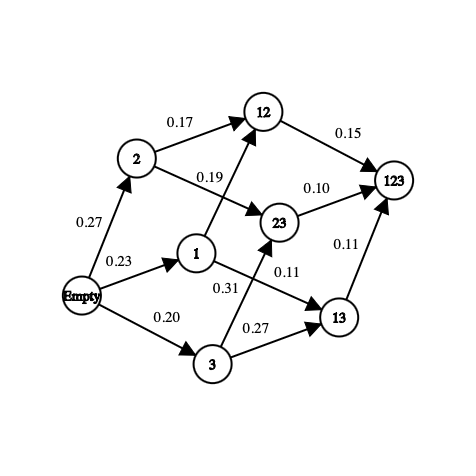
For each state that we visit for the first time a classifier will be trained with the set of features. This value is stored in the state and the training of the classifier, which is very costly, will only happens once even if the state is reached again later. The classifier does not consider the order of the feature. This is why we can see this problem as a graph and not a tree. In this example, the reward of the action of selecting Gender as a new feature for the model is the difference between the accuracy of the current state and the next state.

On the graph above, each feature has been mapped to a number (i.e “Age” is 1, “Gender” is 2 and “Height” is 3). It is totally possible to take other metrics to maximise to find the optimal set. In many business applications the recall is more considered than the accuracy.

The next important question is how do we select the next state from the current state or how do we explore our environement. We have to find the most optimal way to do it since it can quickly become a very complex problem. Indeed, if we naively explore all the possible set of features in a problem with 10 features, the number of states would be

10! + 2 = 3 628 802 possible states

The +2 is because we consider an empty state and a state that contains all the possible features. In this problem we would have to train the same model on all the states to get the set of features that maximises the accuracy. In the RL approach we will not have to go in all the states and to train a model every time that we go in an already visited state.

We had to determine some stop conditions for this problem and they will be detailed later. For now the epsilon-greedy state selection has been chosen. The idea is from a current state we select the next action randomly with a probability of epsilon (between 0 and 1 and often around 0.2) and otherwise select the action that maximises a function. For feature selection the function is the average of reward that each feature has brought to the accuracy of the model.

The epsilon-greedy algorithm implies two steps:

1. A random phase : with a probability epsilon, we select randomly the next state among the possible neighbours of the current state (we can imagine either a uniform or a softmax selection)
2. A greedy phase : we select the next state such that the feature added to the current state has the maximal contribution of accuracy to the model. To reduce the time complexity, we have initialised a list containing this values for each feature. This list is updated every time that a feature is chosen. The update is very optimal thanks to the following formula:

• AORf : Average of reward brought by the feature “f”
• k : number of times that “f” has been selected
• V(F) : state’s value of the set of features F (not detailed in this article for clarity reasons)

The global idea is to find which feature has brought the most accuracy to the model. That is why we need to browse different states to evaluate in many different environments the most global accurate value of a feature for the model.

Finally I will detail the two stop conditions. Since the goal is to minimise the number of state that the algorithm visits we need to be careful about them. The less never visited state we visit, the less amount of models we will have to train with different set of features. Training the model to get the accuracy is the most costly phase in terms of time and computation power.

1. The algorithm stops in any case in the final state which is the set containing all the features. We want to avoid reaching this state since it is the most expensive to train a model with.
2. Also, it stops browsing the graph if a sequence of visited states see their values degrade successively. A threshold has been set such that after square root of the number of total features in the dataset, it stops exploring.

Now that the modelling of the problem has been explained, we will detail the implementation in python.

The python library for Feature Selection with Reinforcement Learning

A python library resolving this problem is available. I will explain in this part how it works and prove that it is an efficient strategy. Also, this article stands as a documentation and you will be able to use this library for your projects by the end of the part.

1. The data pre-processing

Since we need to evaluate the accuracy of a state that is visited, we need to feed a model with the features and the data used for this feature selection task. The data has to been normalised, the categorical variables encoded and have as few rows as possible (the smallest it is, the fastest the algorithm will be). Also, it’s very important to create a mapping between the features and some integers as explained in the previous part. This step is not mandatory but very recommended. The final result of this step is to get a DataFrame with all the features and another with the labels to predict. Below is an example with a dataset used as a benchmark (it can be found here UCI Irvine Machine Learning Repository).

2. Installation and importation of the FSRLearning library

The second step is to install the library with pip. Here is the command to install it:

pip install FSRLearning

To import the library the following code can be used:

You will be able to create a feature selector simply by creating an object Feature_Selector_RL. Some parameters need to be filled in.

• feature_number (integer) : number of features in the DataFrame X
• feature_structure (dictionary) : dictionary for the graph implementation
• eps (float [0; 1]) : probability of choosing a random next state, 0 is an only greedy algorithm and 1 only random
• alpha (float [0; 1]): control the rate of updates, 0 is a very not updating state and 1 a very updated
• gamma (float [0, 1]): factor of moderation of the observation of the next state, 0 is a shortsighted condition and 1 it exhibits farsighted behavior
• nb_iter (int): number of sequences to go through the graph
• starting_state (“empty” or “random”) : if “empty”, the algorithm starts from the empty state and if “random”, the algorithm starts from a random state in the graph

All the parameters can be tuned but for most of the problem only few iterations can be good (around 100) and the epsilon value around 0.2 is often enough. The starting state is useful to browse the graph more efficiently but it can be very dependent on the dataset and both of the values can be tested.

Finally we can initialise very simply the selector with the following code:

Training the algorithm is very easy on the same basis than most of the ML library:

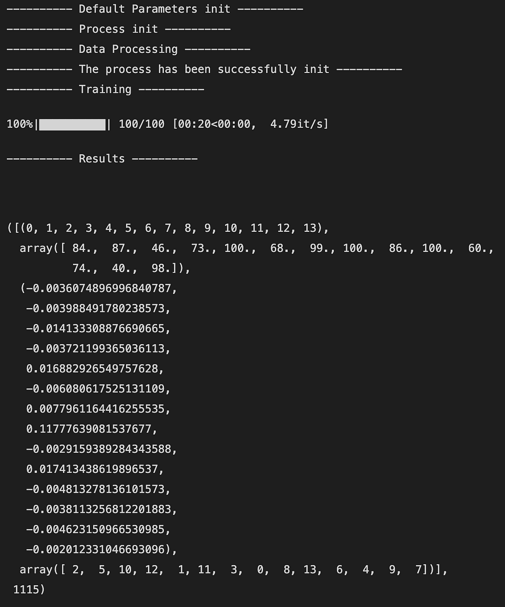
Here is an example of the output:

The output is a 5-tuple as follows:

• Index of the features in the DataFrame X (like a mapping)
• Number or times that the feature has been observed
• Average of reward brought by the feature after all the iterations
• Ranking of the features from the least to the most important (here 2 is the least and 7 the most important feature)
• Number of states globally visited

Another important method of this selector is to get a comparison with the RFE selector of Scikit-Learn. It takes as input X, y and the results of the selector.

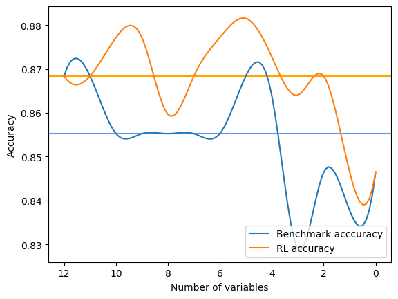
The output is a print after each step of selection of the global metric of RFE and FSRLearning. It also outputs a visual comparison of the accuracy of the model with on the x-axis the number of features selected and on the y-axis the accuracy. The two horizontal lines are the median of accuracy for each method. Here is an example:

Average benchmark accuracy : 0.854251012145749, rl accuracy : 0.8674089068825909 
Median benchmark accuracy : 0.8552631578947368, rl accuracy : 0.868421052631579 
Probability to get a set of variable with a better metric than RFE : 1.0 
Area between the two curves : 0.17105263157894512

In this example the RL method has always given a better set of features for the model than RFE. We can then select with certainty among the sorted set of features any subset and it will give a better accuracy to the model. We can run several times the model and the comparator to get a very accurate estimation but the RL method is always better.

Another interesting method is the get_plot_ratio_exploration. It plots a graph comparing the number of already visited nodes and visited nodes in a sequence for a precise iteration.

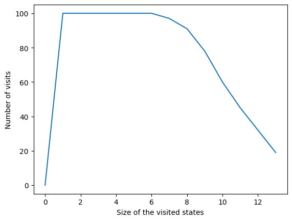
Also, thanks to the second stop condition the time complexity of the algorithm decreases exponentially. Then even if the number of feature is big the convergence will be found quickly. The plot bellow is the number of times that a set of a certain size has been visited.

In all iterations the algorithm visited a state containing 6 variables or less. Beyond 6 variables we can see that the number of state reached is decreasing. It’s a good behaviour since it is faster to train a model with small set of features than the big ones.

Conclusion and references

Overall, we can see that the RL method is very efficient for maximising a metric of a model. It always converges quickly toward an interesting subset of features. Also, this method is very easy and fast to implement in ML projects with the FSRLearning library.

The github repository of the project with a complete documentation is available here.

If you wish to contact me, you can do so directly on linkedin here

This library has been implemented with the help of these two articles:

• Sali Rasoul, Sodiq Adewole and Alphonse Akakpo, FEATURE SELECTION USING REINFORCEMENT LEARNING (2021), ArXiv
• Seyed Mehdin Hazrati Fard, Ali Hamzeh and Sattar Hashemi, Using reinforcement learning to find an optimal set of features (2013), ScienceDirect

Reinforcement Learning for feature selection was originally published in Towards Data Science on Medium, where people are continuing the conversation by highlighting and responding to this story.