Predicting Chicago Taxi Trips with R Time Series Model — BSTS

Predicting Chicago Taxi Trips with R Time Series Model — BSTS

Step-by-step tutorial on how to forecast daily number of taxi trips using R time series model

Introduction

Imaging you’re planning marketing strategies for your taxi company or even considering market entry as a new competitor — predicting number of taxi trips in the big cities can be an interesting business problem. Or, if you’re just a curious resident like me, this article is perfect for you to learn how to use the R Bayesian Structural Time Series (BSTS) model to forecast daily taxi trips and uncover fascinating insights.

In this article, I will walk you through the pipeline including data preparation, explorational data analysis, time series modeling, forecast result analysis, and business insight. I aim to predict the daily number of trips for the second half year of 2023.

Data Preparation

The data was acquired from the Chicago Data Portal. (You will find this platform with access to various government data!) On the website, simply find the “Action” drop down list to query data.

Within the query tool, you’ll find filter, group, and column manager tools. You can simply download the raw dataset. However, to save computing complexity, I grouped the data by pickup timestamp to aggregate the count of trips per 15 minutes.

With exploration of the dataset, I also filtered out the record with 0 trip miles and N/A pickup area code (which means the pickup location is not within Chicago). You should explore the data to decide how you would like to query the data. It should based on the use case of your analysis.

Then, export the processed data. Downloading could take some time !

Exploratory Data Analysis

Understanding the data is the most crucial step to preprocessing and model choices reasoning. In the following part, I dived into different characteristics of the dataset including seasonality, trend, and statistical test for stationary and autocorrelation in the lags.

Seasonality refers to periodic fluctuations in data that occur at regular intervals. These patterns repeat over a specific period, such as days, weeks, months, or quarters.

To understand the seasonality, we first aggregate trip counts by date and month to visualize the effect.

library(lubridate)
library(dplyr)
library(xts)
library(bsts)
library(forecast)
library(tseries)

demand_data <- read.csv("taxi_trip_data.csv")
colnames(demand_data) <- c('trip_cnt','trip_datetime') 
demand_data$trip_datetime <- mdy_hms(demand_data$trip_datetime)
demand_data$rounded_day <- floor_date(demand_data$trip_datetime, unit = "day")
demand_data$rounded_month <- floor_date(demand_data$trip_datetime, unit = "month")

monthly_agg <- demand_data %>%
    group_by(rounded_month) %>%
    summarise(
        trip_cnt = sum(trip_cnt, na.rm = TRUE)
)

daily_agg <- demand_data %>%
    group_by(rounded_day) %>%
    summarise(
        trip_cnt = sum(trip_cnt, na.rm = TRUE)
)

The taxi demand in Chicago peaked in 2014, showed a declining trend with annual seasonality, and was drastically reduced by COVID in 2020.

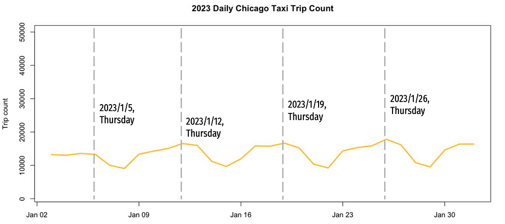
Daily count before COVID suggests weekly seasonality, with higher trip numbers on Fridays and Saturdays.

Interestingly, the post-COVID weekly seasonality has shifted, the Thursdays now have the highest demand. This provides hypothesis about COVID intervention.

Trend in time series data refers to underlying pattern or tendency of the data to increase, decrease, or remain stable over time. I transformed the dataframe to a time series data for STL decomposition to monitor the trend.

zoo_data <- zoo(daily_agg$trip_cnt, order.by = daily_agg$rounded_day)
start_time <- as.numeric(format(index(zoo_data)[1], "%Y"))
ts_data <- ts(coredata(zoo_data), start = start_time, frequency = 365)
stl_decomposition <- stl(ts_data, s.window = "periodic")
plot(stl_decomposition)

The result of STL composition shows that there’s a non-linear trend. The seasonal part also shows a yearly seasonality. After a closer look to the yearly seasonality, I found that Thanksgiving and Christmas have the lowest demand every year.

A time series is considered stationary if its statistical properties (e.g. mean, variance, and autocorrelation) remain constant over time. From the above graphs we already know this data is not stationary since it exhibits trends and seasonality. If you would like to be more robust, ADF and KPSS test are usually leveraged to validate the null hypothesis of non-stationary and stationary respectively.

adf.test(zoo_data)
kpss.test(zoo_data)

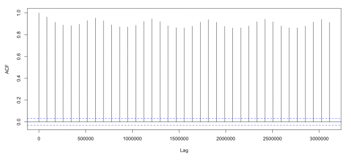
Lag autocorrelation measures the correlation between a time series and its lagged over successive time intervals. It explains how the current value is related to its past values. By autocorrelation in the lags we can identify patterns and help us select appropriate time series models (For example, understanding the autocorrelation structure helps determine the order of AR and MA components for ARIMA model). The graph shows significant autocorrelations at many lags.

acf(zoo_data)

Data Transformation

The EDA provided crucial insights into how we should transform and preprocess the data to achieve the best forecasting results.

COVID changed the time series significantly. It is unreasonable to include data that had changed so much. Here I fit the model on data from 2020 June to 2023 June. This still remains a 6:1 train-test-ratio predicting numbers for the second half of 2023.

train <- window(zoo_data, start = as.Date("2020-07-01"), end = as.Date("2023-06-30"))
test <- window(zoo_data, start = as.Date("2023-07-01"), end = as.Date("2023-12-31"))

The non-stationary data shows huge variance and non-linear trend. Here I applied log and differencing transformation to mitigate the effect of these characteristics on the predicting performance.

train_log <- log(train + 1) 
train_diff <- diff(train, differences = 1)

The following code operates on the log-transformed data, as it yielded better forecasting performance during preliminary tests.

Choosing and Designing the Model

Let’s quickly recap the findings from the EDA:

1. Multiple Seasonality and Non-Linear Trend
2. Impact of Holidays and Events: Significant events like holidays affect taxi demand.
3. Long Prediction Horizon: We need to forecast for 180 days.

Given these characteristics, the Bayesian Structural Time Series (BSTS) model is a suitable choice. The BSTS model decomposes a time series into multiple components using Bayesian methods, capturing the underlying latent variables that evolve over time. The key components typically include:

1. Trend Component
2. Seasonal Component
3. Regressor Component: Incorporates the influence of external variables that might affect the time series.

This is the model I used to predict the taxi trips:

ss <- AddSemilocalLinearTrend(list(), train_log) 
ss <- AddSeasonal(ss, train_log, nseasons = 7)
ss <- AddSeasonal(ss, train_log, nseasons = 365)
ss <- AddMonthlyAnnualCycle(ss, train_log)
ss <- AddRegressionHoliday(ss, train_log, holiday_list)
model_log_opti <- bsts(train_log, state.specification = ss, niter = 5000, verbose = TRUE, seed=1014)
summary(model_log_opti)

AddSemilocalLinearTrend()
From the EDA, the trend in our data is not a random walk. Therefore, we use a semi-local linear trend, which assumes the level component moves according to a random walk, but the slope component follows an AR1 process centered on a potentially non-zero value. This is useful for long-term forecasting.

AddSeasonal()
The seasonal model can be thought of as a regression on nseasons dummy variables. Here we include weekly and yearly seasonality by setting nseasons to 7 and 365.

AddMonthlyAnnualCycle()
This represents the contribution of each month. Alternatively, you can set nseasons=12 in AddSeasonal() to address monthly seasonality.

AddRegressionHoliday()
Previously in EDA we learned that Thanksgiving and Christmas negatively impact taxi trips. This function estimate the effect of each holiday or events using regression. For this, I asked a friend of mine who is familiar with Chicago (well, ChatGPT of course) for the list of huge holidays and events in Chicago. For example, the Chicago Marathon might boost the number of taxi trips.

Then I set up the date of these dates:

christmas <- NamedHoliday("Christmas")
new_year <- NamedHoliday("NewYear")
thanksgiving <- NamedHoliday("Thanksgiving")
independence_day <- NamedHoliday("IndependenceDay")
labor_day <- NamedHoliday("LaborDay")
memorial_day <- NamedHoliday("MemorialDay")

auto.show <- DateRangeHoliday("Auto_show", start = as.Date(c("2013-02-09", "2014-02-08", "2015-02-14", "2016-02-13", "2017-02-11"
                                                             , "2018-02-10", "2019-02-09", "2020-02-08", "2021-07-15", "2022-02-12"
                                                             , "2023-02-11")), 
                              end = as.Date(c("2013-02-18", "2014-02-17", "2015-02-22", "2016-02-21", "2017-02-20"
                                                , "2018-02-19", "2019-02-18", "2020-02-17"
                                                , "2021-07-19", "2022-02-21", "2023-02-20")))
st.patrick <- DateRangeHoliday("stPatrick", start = as.Date(c("2013/3/16", "2014/3/15", "2015/3/14", "2016/3/12"
                                                              , "2017/3/11", "2018/3/17", "2019/3/16", "2020/3/14"
                                                              , "2021/3/13", "2022/3/12", "2023/3/11")), 
                              end = as.Date(c("2013/3/16", "2014/3/15", "2015/3/14", "2016/3/12"
                                                              , "2017/3/11", "2018/3/17", "2019/3/16", "2020/3/14"
                                                              , "2021/3/13", "2022/3/12", "2023/3/11")))
air.show <- DateRangeHoliday("air_show", start = as.Date(c("2013/8/17", "2014/8/16", "2015/8/15", "2016/8/20"
                                                           , "2017/8/19", "2018/8/18", "2019/8/17"
                                                           , "2021/8/21", "2022/8/20", "2023/8/19")), 
                              end = as.Date(c("2013/8/18", "2014/8/17", "2015/8/16", "2016/8/21", "2017/8/20"
                                              , "2018/8/19", "2019/8/18", "2021/8/22", "2022/8/21", "2023/8/20")))
lolla <- DateRangeHoliday("lolla", start = as.Date(c("2013/8/2", "2014/8/1", "2015/7/31", "2016/7/28", "2017/8/3"
                                                     , "2018/8/2", "2019/8/1", "2021/7/29", "2022/7/28", "2023/8/3")), 
                              end = as.Date(c("2013/8/4", "2014/8/3", "2015/8/2", "2016/7/31", "2017/8/6", "2018/8/5"
                                              , "2019/8/4", "2021/8/1", "2022/7/31", "2023/8/6")))
marathon <- DateRangeHoliday("marathon", start = as.Date(c("2013/10/13", "2014/10/12", "2015/10/11", "2016/10/9", "2017/10/8"
                                                        , "2018/10/7", "2019/10/13", "2021/10/10", "2022/10/9", "2023/10/8")), 
                              end = as.Date(c("2013/10/13", "2014/10/12", "2015/10/11", "2016/10/9", "2017/10/8"
                                                        , "2018/10/7", "2019/10/13", "2021/10/10", "2022/10/9", "2023/10/8")))

DateRangeHoliday() allows us to define events that happen at different date each year or last for multiple days. NameHoliday() helps with federal holidays.

Then, define the list of these holidays for the AddRegressionHoliday() attribute:

holiday_list <- list(auto.show, st.patrick, air.show, lolla, marathon
              , christmas, new_year, thanksgiving, independence_day
              , labor_day, memorial_day)

I found this website very helpful in exploring different component and parameters.

The fitted result shows that the model well captured the component of the time series.

fitted_values <- as.numeric(residuals.bsts(model_log_opti, mean.only=TRUE)) + as.numeric(train_log)
train_hat <- exp(fitted_values) - 1
plot(as.numeric(train), type = "l", col = "blue", ylim=c(500, 30000), main="Fitted result")
lines(train_hat, col = "red")
legend("topleft", legend = c("Actual value", "Fitted value"), col = c("blue", "red"), lty = c(1, 1), lwd = c(1, 1))

In the residual analysis, although the residuals have a mean of zero, there is still some remaining seasonality. Additionally, the residuals exhibit autocorrelation in the first few lags.

However, when comparing these results to the original time series, it is evident that the model has successfully captured most of the seasonality, holiday effects, and trend components. This indicates that the BSTS model effectively addresses the key patterns in the data, leaving only minor residual structures to be examined further.

Forecast Result and Insights

Now, let’s evaluate the forecast results of the model. Remember to transform the predicted values, as the model provides logged values.

horizon <- length(test)
pred_log_opti <- predict(model_log_opti, horizon = horizon, burn = SuggestBurn(.1, ss))
forecast_values_log_opti <- exp(pred_log_opti$mean) - 1

plot(as.numeric(test), type = "l", col = "blue", ylim=c(500, 30000), main="Forecast result", xlab="Time", ylab="Trip count")
lines(forecast_values_log_opti, col = "red")
legend("topleft", legend = c("Actual value", "Forecast value"), col = c("blue", "red"), lty = c(1, 1), lwd = c(1, 1))

The model achieves a Mean Absolute Percentage Error (MAPE) of 9.76%, successfully capturing the seasonality and the effects of holidays.

The analysis of holiday and event effects offers valuable insights for business strategies. The following graphs illustrate the impact of holiday regressions:

PlotHoliday(thanksgiving, model_log_opti)
PlotHoliday(marathon, model_log_opti)

The day before federal holidays has a significantly negative impact on the number of trips. For example, both Thanksgiving Day and the day before show a noticeable drop in taxi trips. This reduction could be due to lower demand or limited supply. Companies can investigate these reasons further and develop strategies to address them.

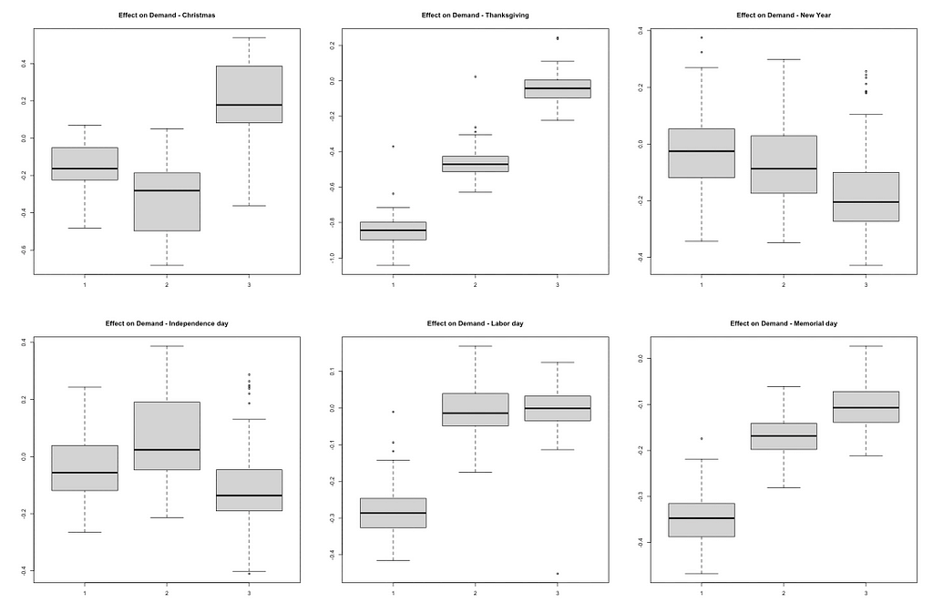
Contrary to the initial hypothesis, major events like the Chicago Marathon did not show a significant increase in taxi demand. This suggests that demand during such events may not be as high as expected. Conducting customer segmentation research can help identify specific groups that might be influenced by events, revealing potential opportunities for targeted marketing and services. Breaking down the data by sub-areas in Chicago can also provide better insights. The impact of events might vary across different neighborhoods, and understanding these variations can help tailor localized strategies.

Conclusion

So this is how you can use BSTS model to predict Chicago taxi rides! You can experiment different state component or parameters to see how the model fit the data differently. Hope you enjoy the process and please give me claps if you find this article helpful!

---

Predicting Chicago Taxi Trips with R Time Series Model — BSTS was originally published in Towards Data Science on Medium, where people are continuing the conversation by highlighting and responding to this story.