Powering Experiments with CUPED and Double Machine Learning

Causal AI, exploring the integration of causal reasoning into machine learning

What is this series of articles about?

Welcome to my series on Causal AI, where we will explore the integration of causal reasoning into machine learning models. Expect to explore a number of practical applications across different business contexts.

In the last article we covered safeguarding demand forecasting with causal graphs. Today, we turn our attention to powering experiments using CUPED and double machine learning.

If you missed the last article on safeguarding demand forecasting, check it out here:

Safeguarding Demand Forecasting with Causal Graphs

Introduction

In this article, we evaluate whether CUPED and double machine learning can enhance the effectiveness of your experiments. We will use a case study to explore the following areas:

• The building blocks of experimentation: Hypothesis testing, power analysis, bootstrapping.
• What is CUPED and how can it help power experiments?
• What are the conceptual similarities between CUPED and double machine learning?
• When should we use double machine learning rather than CUPED?

The full notebook can be found here:

causal_ai/notebooks/powering your experiments – cuped.ipynb at main · raz1470/causal_ai

Case study

Background

You’ve recently joined the experimentation team at a leading online retailer known for its vast product catalog and dynamic user base. The data science team has deployed an advanced recommender system designed to enhance user experience and drive sales. This system integrates in real-time with the retailer’s platform and involves significant infrastructure and engineering costs.

The finance team is eager to understand the system’s financial impact, specifically how much additional revenue it generates compared to a baseline scenario without recommendations. To evaluate the recommender system’s effectiveness, you plan to conduct a randomized controlled experiment.

Data-generating process: Pre-experiment

We start by creating some pre-experiment data. The data-generating process we use has the following characteristics:

• 3 observed covariates related to the recency (x_recency), frequency (x_frequency) and value (x_value) of previous sales.
• 1 unobserved covariate, the users monthly income (u_income).

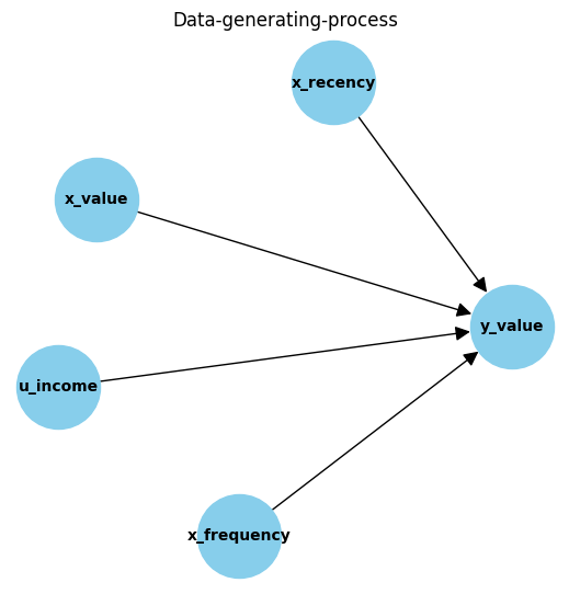
• A complex relationship between covariates is used to estimate our target metric, sales value:

The python code below is used to create the pre-experiment data:

np.random.seed(123)

n = 10000 # Set number of observations
p = 4 # Set number of pre-experiment covariates

# Create pre-experiment covariates
X = np.random.uniform(size=n * p).reshape((n, -1))

# Nuisance parameters
b = (
    1.5 * X[:, 0] +
    2.5 * X[:, 1] +
    X[:, 2] ** 3 +     
    X[:, 3] ** 2 +
    X[:, 1] * X[:, 2]  
)

# Create some noise
noise = np.random.normal(size=n)

# Calculate outcome
y = np.maximum(b + noise, 0)

# Scale variables for interpretation
df_pre = pd.DataFrame({"noise": noise * 1000,
                   "u_income": X[:, 0] * 1000,                   
                   "x_recency": X[:, 1] * 1000,
                   "x_frequency": X[:, 2] * 1000,
                   "x_value": X[:, 3] * 1000,
                   "y_value": y * 1000     
})

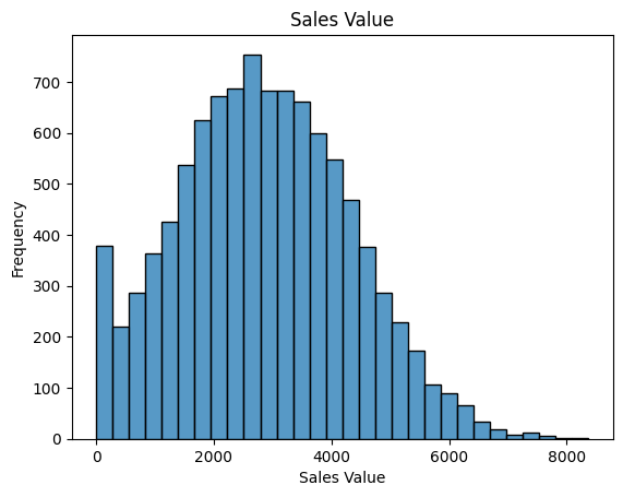
# Visualise target metric
sns.histplot(df_pre['y_value'], bins=30, kde=False)
plt.xlabel('Sales Value')
plt.ylabel('Frequency')
plt.title('Sales Value')
plt.show()

The building blocks of experimentation: Hypothesis testing, power analysis, bootstrapping

Before we get onto CUPED, I thought it would be worthwhile covering some foundational knowledge on experimentation.

Hypothesis testing

Hypothesis testing helps determine if observed differences in an experiment are statistically significant or just random noise. In our experiment, we divide users into two groups:

• Control Group: Receives no recommendations.
• Treatment Group: Receives personalised recommendations from the system.

We define our hypotheses as follows:

• Null Hypothesis (H₀): The recommender system does not affect revenue. Any observed differences are due to chance.
• Alternative Hypothesis (Hₐ): The recommender system increases revenue. Users receiving recommendations generate significantly more revenue compared to those who do not.

To assess the hypotheses you will be comparing the mean revenue in the control and treatment group. However, there are a few things to be aware of:

• Type I error (False positive): If the experiment concludes that the recommender system significantly increases revenue when in reality, it has no effect.
• Type II error (Beta, False negative): If the experiment finds no significant increase in revenue from the recommender system when in reality, it does lead to a meaningful increase
• Significance Level (Alpha): If you set the significance level to 0.05, you are accepting a 5% chance of incorrectly concluding that the recommender system improves revenue when it does not (false positive).
• Power (1 — Beta): Achieving a power of 0.80 means you have an 80% chance of detecting a significant increase in revenue due to the recommender system if it truly has an effect. A higher power reduces the risk of false negatives.

As you start to think about designing the experiment, you set some initial goals:

1. You want to reliably detect the effect — Making sure you balance the risks of detecting a non-existent effect vs the risk of not detecting a real effect.
2. As quickly as possible — Finance are on your case!
3. Keeping the sample size as cost efficient as possible — The business case from the data science team suggests the system is going to drive a large increase in revenue so they don’t want the control group being too big.

But how can you meet these goals? Let’s delve into power analysis next!

Power analysis

When we talk about powering experiments, we are usually referring to the process of determining the minimum sample size needed to detect an effect of a certain size with a given confidence. There are 3 components to power analysis:

• Effect size — The difference between the mean value of H₀ and Hₐ. We generally need to make sensible assumptions around this based on understanding what matters to the business/industry we are operating within.
• Significance level — The probability of incorrectly concluding there is an effect when there isn’t, typically set at 0.05.
• Power — The probability of correctly detecting an effect when there is one, typically set at 0.80.

I found the intuition behind these quite hard to grasp at first, but visualising it can really help. So lets give it a try! The key areas are where H₀ and Hₐ crossover — See if you it helps you tie together the components discussed above…

A larger sample size leads to a smaller standard error. With a smaller standard error, the sampling distributions of H₀ and Hₐ become narrower and less overlapping. This decreased overlap makes it easier to detect a difference, leading to higher power.

The function below shows how we can use the statsmodels python package to carry out a power analysis:

from typing import Union
import pandas as pd
import numpy as np
import statsmodels.stats.power as smp

def power_analysis(metric: Union[np.ndarray, pd.Series], exp_perc_change: float, alpha: float = 0.05, power: float = 0.80) -> int:
    '''
    Perform a power analysis to determine the minimum sample size required for a given metric.

    Args:
        metric (np.ndarray or pd.Series): Array or Series containing the metric values for the control group.
        exp_perc_change (float): The expected percentage change in the metric for the test group.
        alpha (float, optional): The significance level for the test. Defaults to 0.05.
        power (float, optional): The desired power of the test. Defaults to 0.80.

    Returns:
        int: The minimum sample size required for each group to detect the expected percentage change with the specified power and significance level.

    Raises:
        ValueError: If `metric` is not a NumPy array or pandas Series.
    '''
    
    # Validate input types
    if not isinstance(metric, (np.ndarray, pd.Series)):
        raise ValueError("metric should be a NumPy array or pandas Series.")
    
    # Calculate statistics
    control_mean = metric.mean()
    control_std = np.std(metric, ddof=1) # Use ddof=1 for sample standard deviation
    test_mean = control_mean * (1 + exp_perc_change)
    test_std = control_std # Assume the test group has the same standard deviation as the control group
    
    # Calculate (Cohen's D) effect size
    mean_diff = control_mean - test_mean
    pooled_std = np.sqrt((control_std**2 + test_std**2) / 2)
    effect_size = abs(mean_diff / pooled_std)  # Cohen's d should be positive
    
    # Run power analysis
    power_analysis = smp.TTestIndPower()
    sample_size = round(power_analysis.solve_power(effect_size=effect_size, alpha=alpha, power=power))
    
    print(f"Control mean: {round(control_mean, 3)}")
    print(f"Control std: {round(control_std, 3)}")
    print(f"Min sample size: {sample_size}")
    
    return sample_size

So let’s test it out with our pre-experiment data!

exp_perc_change = 0.05 # Set the expected percentage change in the chosen metric caused by the treatment

min_sample_size = power_analysis(df_pre["y_value"], exp_perc_change

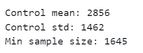
We can see that given the distribution of our target metric, we would need a sample size of 1,645 to detect an increase of 5%.

Data-generating process: Experimental data

Rather than rush into setting up the experiment, you decide to take the pre-experiment data and simulate the experiment.

The following function randomly selects users to be treated and applies a treatment effect. At the end of the function we record the mean difference before and after the treatment was applied as well as the true ATE (average treatment effect):

def exp_data_generator(t_perc_change, t_samples):

    # Create copy of pre-experiment data ready to manipulate into experiment data
    df_exp = df_pre.reset_index(drop=True)

    # Calculate the initial treatment effect
    treatment_effect = round((df_exp["y_value"] * (t_perc_change)).mean(), 2)

    # Create treatment column
    treated_indices = np.random.choice(df_exp.index, size=t_samples, replace=False)
    df_exp["treatment"] = 0
    df_exp.loc[treated_indices, "treatment"] = 1

    # treatment effect
    df_exp["treatment_effect"] = 0
    df_exp.loc[df_exp["treatment"] == 1, "treatment_effect"] = treatment_effect

    # Apply treatment effect
    df_exp["y_value_exp"] = df_exp["y_value"] 
    df_exp.loc[df_exp["treatment"] == 1, "y_value_exp"] = df_exp["y_value"] + df_exp["treatment_effect"]

    # Calculate mean diff before treatment
    mean_t0_pre = df_exp[df_exp["treatment"] == 0]["y_value"].mean()
    mean_t1_pre = df_exp[df_exp["treatment"] == 1]["y_value"].mean()
    mean_diff_pre  = round(mean_t1_pre  - mean_t0_pre)

    # Calculate mean diff after treatment
    mean_t0_post = df_exp[df_exp["treatment"] == 0]["y_value_exp"].mean()
    mean_t1_post = df_exp[df_exp["treatment"] == 1]["y_value_exp"].mean()
    mean_diff_post  = round(mean_t1_post  - mean_t0_post)

    # Calculate ate
    treatment_effect = round(df_exp[df_exp["treatment"]==1]["treatment_effect"].mean())

    print(f"Diff-in-means before treatment: {mean_diff_pre}")
    print(f"Diff-in-means after treatment: {mean_diff_post}")
    print(f"ATE: {treatment_effect}")
    
    return df_exp

We can feed through the minimum sample size we previously calculated:

np.random.seed(123)
df_exp_1 = exp_data_generator(exp_perc_change, min_sample_size)

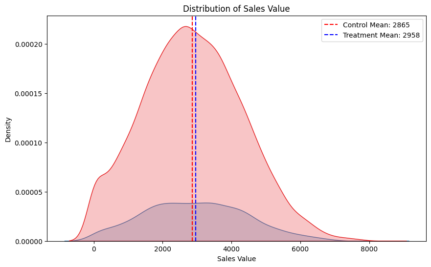
Let’s start by inspecting the data we created for treated users to help you understand what the function is doing:

Next let’s take a look at the results which the function prints:

Interesting, we see that after we select users to be treated, but before we treat them, there is already a difference in means. This difference is due to chance. This means that when we look at the difference after users are treated we don’t correctly estimate the ATE (average treatment effect). We will come back to this point when we cover CUPED.

Next let’s explore a more sophisticated way of making an inference than just taking the difference in means…

Bootstrapping

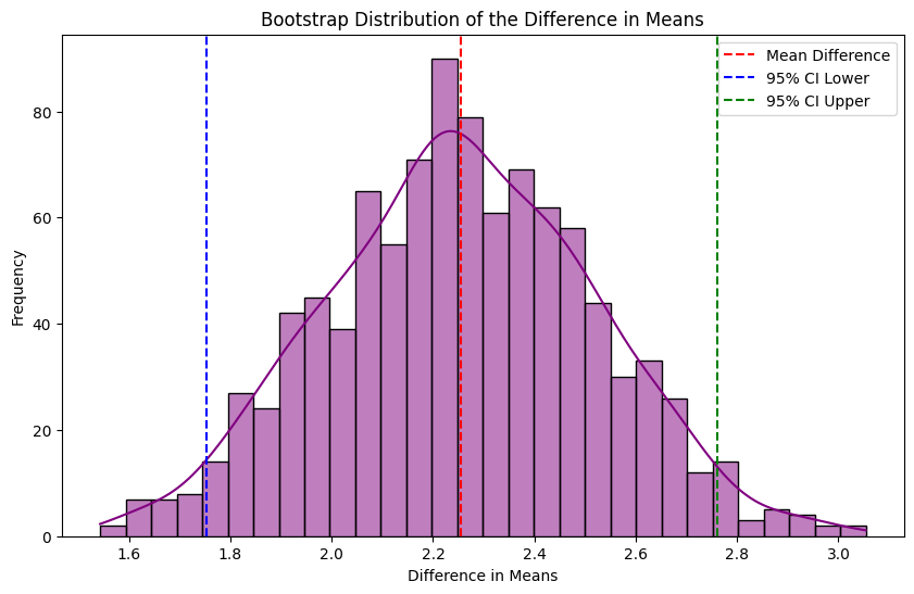
Bootstrapping is a powerful statistical technique that involves resampling data with replacement. These resampled datasets, called bootstrap samples, help us estimate the variability of a statistic (like the mean or median) from our original data. This is particularly attractive when it comes to experimentation as it enables us to calculate confidence intervals. Let’s walk through it step by step using a simple example…

You have run an experiment with a control and treatment group each made up of 1k users.

1. Create bootstrap samples — Randomly select (with replacement) 1k users from the control and then treatment group. This gives us 1 bootstrap sample for control and one for treatment.
2. Repeat this process n times (e.g. 10k times).
3. For each pair of bootstrap samples calculate the mean difference between control and treatment.
4. We now have a distribution (made up of the mean difference between 10k bootstrap samples) which we can use to calculate confidence intervals.

Applying it to our case study

Let’s use our case study to illustrate how it works. Below we use the sciPy stats python package to help calculate bootstrap confidence intervals:

from typing import Union
import pandas as pd
import numpy as np
from scipy import stats

def mean_diff(group_a: Union[np.ndarray, pd.Series], group_b: Union[np.ndarray, pd.Series]) -> float:
    '''
    Calculate the difference in means between two groups.

    Args:
        group_a (Union[np.ndarray, pd.Series]): The first group of data points.
        group_b (Union[np.ndarray, pd.Series]): The second group of data points.

    Returns:
        float: The difference between the mean of group_a and the mean of group_b.
    '''
    return np.mean(group_a) - np.mean(group_b)

def bootstrapping(df: pd.DataFrame, adjusted_metric: str, n_resamples: int = 10000) -> np.ndarray:
    '''
    Perform bootstrap resampling on the adjusted metric of two groups in the dataframe to estimate the mean difference and confidence intervals.

    Args:
        df (pd.DataFrame): The dataframe containing the data. Must include a 'treatment' column indicating group membership.
        adjusted_metric (str): The name of the column in the dataframe representing the metric to be resampled.
        n_resamples (int, optional): The number of bootstrap resamples to perform. Defaults to 1000.

    Returns:
        np.ndarray: The array of bootstrap resampled mean differences.
    '''
    
    # Separate the data into two groups based on the 'treatment' column
    group_a = df[df["treatment"] == 1][adjusted_metric]
    group_b = df[df["treatment"] == 0][adjusted_metric]

    # Perform bootstrap resampling
    res = stats.bootstrap((group_a, group_b), statistic=mean_diff, n_resamples=n_resamples, method='percentile')
    ci = res.confidence_interval
    
    # Extract the bootstrap distribution and confidence intervals
    bootstrap_means = res.bootstrap_distribution
    bootstrap_ci_lb = round(ci.low,)
    bootstrap_ci_ub = round(ci.high)    
    bootstrap_mean = round(np.mean(bootstrap_means))

    print(f"Bootstrap confidence interval lower bound: {bootstrap_ci_lb}")
    print(f"Bootstrap confidence interval upper bound: {bootstrap_ci_ub}")    
    print(f"Bootstrap mean diff: {bootstrap_mean}")
    
    return bootstrap_means

When we run it for our case study data we can see that we now have some confidence intervals:

bootstrap_og_1 = bootstrapping(df_exp_1, "y_value_exp")

Our ground truth ATE is 143 (the actual treatment effect from our experiment data generator function), which falls within our confidence intervals. However, it’s worth noting that the mean difference hasn’t changed (it’s still 93 as before when we simply calculated the mean difference of control and treatment), and the pre-treatment difference is still there.

So what if we wanted to come up with narrower confidence intervals? And is there any way we can deal with the pre-treatment differences? This leads us nicely into CUPED…

What is CUPED and how can it help power experiments?

Background

CUPED (controlled experiments using pre-experiment data) is a powerful technique for improving the accuracy of experiments developed by researchers at Microsoft. The original paper is an insightful read for anyone interested in experimentation:

https://ai.stanford.edu/~ronnyk/2009controlledExperimentsOnTheWebSurvey.pdf

The core idea of CUPED is to use data collected before your experiment begins to reduce the variance in your target metric. By doing so, you can make your experiment more sensitive, which has two major benefits:

1. You can detect smaller effects with the same sample size.
2. You can detect the same effect with a smaller sample size.

Think of it like removing the “background noise” so you can see the “signal” more clearly.

Variance, standard deviation, standard error

When you read about CUPED you may hear people talk about it reducing the variance, standard deviation or standard error. If you are anything like me, you might find yourself forgetting how these are related, so before we go any further let’s recap on this!

• Variance: Variance measures the average squared deviation of each data point from the mean, reflecting the overall spread or dispersion within a dataset.
• Standard Deviation: Standard deviation is the square root of variance, representing the average distance of each data point from the mean, and providing a more interpretable measure of spread.
• Standard Error: Standard error quantifies the precision of the sample mean as an estimate of the population mean, calculated as the standard deviation divided by the square root of the sample size.

How does CUPED work?

To understand how CUPED works, let’s break it down…

Pre-experiment covariate — In the lightest implementation of CUPED, the pre-experiment covariate would be the target metric measured in a time period before the experiment. So if your target metric was sales value, your covariate could be each customers sales value 4 weeks prior to the experiment.

It’s important that your covariate is correlated with your target metric and that it is unaffected by the treatment. This is why we would typically use pre-treatment data from the control group.

Regression adjustment — Linear regression is used to model the relationship between the covariate (measured before the experiment) and the target metric (measured across the experiment period). We can then calculate the CUPED adjusted target metric by removing the influence of the covariate:

It is worth noting that taking away the mean of the covariate is done to centre the outcome variable around the mean to make it interpretable when compared to the original target metric.

Variance reduction — After the regression adjustment the variance in our target metric has reduced. Lower variance means that the differences between the control and treatment group are easier to detect, thus increasing the statistical power of the experiment.

Applying it to our case study

Let’s use our case study to illustrate how it works. Below we code CUPED up in a function:

from typing import Union
import pandas as pd
import numpy as np
import statsmodels.api as sm

def cuped(df: pd.DataFrame, pre_covariates: Union[str, list], target_metric: str) -> pd.Series:
    '''
    Implements the CUPED (Controlled Experiments Using Pre-Experiment Data) technique to adjust the target metric 
    by removing predictable variation using pre-experiment covariates. This reduces the variance of the metric and 
    increases the statistical power of the experiment.

    Args:
        df (pd.DataFrame): The input DataFrame containing both the pre-experiment covariates and the target metric. 
        pre_covariates (Union[str, list]): The column name(s) in the DataFrame corresponding to the pre-experiment covariates used for the adjustment. 
        target_metric (str): The column name in the DataFrame representing the metric to be adjusted.

    Returns:
        pd.Series: A pandas Series containing the CUPED-adjusted target metric.
    '''
    
    # Fit control model using pre-experiment covariates
    control_group = df[df['treatment'] == 0]
    X_control = control_group[pre_covariates]
    X_control = sm.add_constant(X_control)
    y_control = control_group[target_metric]
    model_control = sm.OLS(y_control, X_control).fit()

    # Compute residuals and adjust target metric
    X_all = df[pre_covariates]
    X_all = sm.add_constant(X_all)
    residuals = df[target_metric].to_numpy().flatten() - model_control.predict(X_all)
    adjustment_term = model_control.params['const'] + sum(model_control.params[covariate] * df[pre_covariates].mean()[covariate] for covariate in pre_covariates)
    adjusted_target = residuals + adjustment_term
    
    return adjusted_target

When we apply it to our case study data and compare the adjusted target metric to the original target metric, we see that the variance has reduced:

# Apply CUPED
pre_covariates = ["x_recency", "x_frequency", "x_value"]
target_metric = ["y_value_exp"]
df_exp_1["adjusted_target"] = cuped(df_exp_1, pre_covariates, target_metric)

# Plot results
plt.figure(figsize=(10, 6))
sns.kdeplot(data=df_exp_1[df_exp_1['treatment'] == 0], x="adjusted_target", hue="treatment", fill=True, palette="Set1", label="Adjusted Value")
sns.kdeplot(data=df_exp_1[df_exp_1['treatment'] == 0], x="y_value_exp", hue="treatment", fill=True, palette="Set2", label="Original Value")
plt.title(f"Distribution of Value by Original vs CUPED")
plt.xlabel("Value")
plt.ylabel("Density")
plt.legend(title="Distribution")

Does it reduce the standard error?

Now we have applied CUPED and reduced the variance, lets run our bootstrapping function to see what impact it has:

bootstrap_cuped_1 = bootstrapping(df_exp_1, "adjusted_target")

If you compare this to our previous result using the original target metric you see that the confidence intervals are narrower:

bootstrap_1 = pd.DataFrame({
    'original': bootstrap_og_1,
    'cuped': bootstrap_cuped_1
})

# Plot the KDE plots
plt.figure(figsize=(10, 6))
sns.kdeplot(bootstrap_1['original'], fill=True, label='Original', color='blue')
sns.kdeplot(bootstrap_1['cuped'], fill=True, label='CUPED', color='orange')

# Add mean lines
plt.axvline(bootstrap_1['original'].mean(), color='blue', linestyle='--', linewidth=1)
plt.axvline(bootstrap_1['cuped'].mean(), color='orange', linestyle='--', linewidth=1)
plt.axvline(round(df_exp_1[df_exp_1["treatment"]==1]["treatment_effect"].mean(), 3), color='green', linestyle='--', linewidth=1, label='Treatment effect')

# Customize the plot
plt.title('Distribution of Value by Original vs CUPED')
plt.xlabel('Value')
plt.ylabel('Density')
plt.legend()

# Show the plot
plt.show()

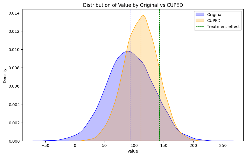
The bootstrap difference in means also moves closer to the ground truth treatment effect. This is because CUPED is also very effective at dealing with pre-existing differences between the control and treatment group.

Does it reduce the minimum sample size?

The next question is does it reduce the minimum sample size we need. Well lets find out!

treatment_effect_1 = round(df_exp_1[df_exp_1["treatment"]==1]["treatment_effect"].mean(), 2)
cuped_sample_size = power_analysis(df_exp_1[df_exp_1['treatment'] == 0]['adjusted_target'], treatment_effect_1 / df_exp_1[df_exp_1['treatment'] == 0]['adjusted_target'].mean())

The minimum sample size needed has reduced from 1,645 to 901. Both Finance and the Data Science team are going to be pleased as we can run the experiment for a shorter time period with a smaller control sample!

What are the conceptual similarities between CUPED and double machine learning?

Background

When I first read about CUPED, I thought of double machine learning and the similarities. If you aren’t familiar with double machine learning, check out my article from earlier in the series:

De-biasing Treatment Effects with Double Machine Learning

Pay attention to the first stage outcome model in double machine learning:

• Outcome model (de-noising): Machine learning model used to estimate the outcome using just the control features. The outcome model residuals are then calculated.

This is conceptually very similar to what we are doing with CUPED!

How does it compare to CUPED?

Let’s feed through our case study data and see if we get a similar result:

# Train DML model
dml = LinearDML(discrete_treatment=False)
dml.fit(df_exp_1[target_metric].to_numpy().ravel(), T=df_exp_1['treatment'].to_numpy().ravel(), X=df_exp_1[pre_covariates], W=None)
ate_dml = round(dml.ate(df_exp_1[pre_covariates]))
ate_dml_lb = round(dml.ate_interval(df_exp_1[pre_covariates])[0])
ate_dml_ub = round(dml.ate_interval(df_exp_1[pre_covariates])[1])

print(f'DML confidence interval lower bound: {ate_dml_lb}')
print(f'DML confidence interval upper bound: {ate_dml_ub}')
print(f'DML ate: {ate_dml}')

We get an almost identical result!

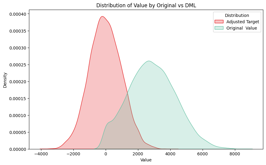
When we plot the residuals we can see that the variance is reduced like in CUPED (although we don’t add the mean to scale for interpretation):

# Fit model outcome model using pre-experiment covariates
X_all = df_exp_1[pre_covariates]
X_all = sm.add_constant(X)
y_all = df_exp_1[target_metric]
outcome_model = sm.OLS(y_all, X_all).fit()

# Compute residuals and adjust target metric
df_exp_1['outcome_residuals'] = df_exp_1[target_metric].to_numpy().flatten() - outcome_model.predict(X_all)

# Plot results
plt.figure(figsize=(10, 6))
sns.kdeplot(data=df_exp_1[df_exp_1['treatment'] == 0], x="outcome_residuals", hue="treatment", fill=True, palette="Set1", label="Adjusted Target")
sns.kdeplot(data=df_exp_1[df_exp_1['treatment'] == 0], x="y_value_exp", hue="treatment", fill=True, palette="Set2", label="Original  Value")
plt.title(f"Distribution of Value by Original vs DML")
plt.xlabel("Value")
plt.ylabel("Density")
plt.legend(title="Distribution")

plt.show()

“So what?” I hear you ask!

Firstly, I think it’s an interesting observation for anyone using double machine learning — The first stage outcome model help reduce the variance and therefore we should get similar benefits to CUPED.

Secondly, it raises the question when is each method appropriate? Let’s close things off by covering off this question…

When should we use double machine learning rather than CUPED?

There are several reasons why it may make sense to tend towards CUPED:

• It’s easier to understand.
• It’s simpler to implement.
• It’s one model rather than three, meaning you have less challenges with overfitting.

However, there are a couple of exceptions where double machine learning outperforms CUPED:

• Biased treatment assignment — When the treatment assignment is biased, for example when you are using observational data, double machine learning can deal with this. My article from earlier in the series builds on this:

De-biasing Treatment Effects with Double Machine Learning

• Heterogenous treatment effects — When you want to understand effects at an individual level, for example finding out who it is worth sending discounts to, double machine learning can help with this. There is a good case study which illustrates this in my previous article on optimising treatment strategies:

Using Double Machine Learning and Linear Programming to optimise treatment strategies

Final thoughts

Today we did a whistle stop tour of experimentation, covering hypothesis testing, power analysis and bootstrapping. We then explored how CUPED can reduce the standard error and increase the power of our experiments. Finally, we touched on it’s similarities to double machine learning and discussed when each method should be used. There are a few additional key points which are worth mentioning in terms CUPED:

• We don’t have to use linear regression — If we have multiple covariates, maybe some with non-linear relationships, we could use a machine learning technique like boosting.
• If we do go down the route of using a machine learning technique, we need to make sure not to overfit the data.
• Some careful thought should go into when to run CUPED — Are you going to run it before you start your experiment and then run a power analysis to determine your reduced sample size? Or are you just going to run it after your experiment to reduce the standard error?

Follow me if you want to continue this journey into Causal AI – In the next article we will find out why Diff-in-Diffs is taking the world by storm!

Powering Experiments with CUPED and Double Machine Learning was originally published in Towards Data Science on Medium, where people are continuing the conversation by highlighting and responding to this story.