Large transaction volumes have soared by 2004% in the past 24 hours.
Currently, 67.16% of top traders hold long positions, while 32.84% hold short positions.
Why Bayesian A/B testing can lead to misunderstandings, inflated false positive rates, introduce bias and complicate results
(Image generated by the author using Midjourney)
Over the past decade, I’ve engaged in countless discussions about Bayesian A/B testing versus Frequentist A/B testing. In nearly every conversation, I’ve maintained the same viewpoint: there’s a significant disconnect between the industry’s enthusiasm for Bayesian testing and its actual contribution, validity, and effectiveness. While the hype around Bayesian testing may have peaked, it remains widely popular.
My first exposure to Bayesian statistics was during my master’s studies, where my thesis focused on Thompson Sampling. Professionally, I encountered Bayesian A/B testing during my tenure at Wix.com, where I played a key role in transitioning from the classical method to the Bayesian method. My perspective, as described here, has been informed by both my academic background and my professional experience at Wix and beyond, where I’ve helped many companies enhance their A/B testing capabilities.
When referring to “Bayesian A/B testing”, I’m specifically talking about the methods promoted by VWO and similar approaches used in some current experimentation platforms as alternatives to the classic (Frequentist) method. There are other implementations of Bayesian statistics in A/B testing, such as Thompson sampling in Multi-armed-bandit experiments, which can be highly effective but are rare outside marketing platforms like Google Ads and Facebook Ads.
In this post, I’ll explain what Bayesian tests entail, outline the most common arguments in favor of Bayesian tests, and address each argument. I’ll then discuss the major drawbacks of the Bayesian method and, finally, cover when to use Bayesian methods in experiments.
So grab a cup of coffee, and let’s dive in.
What Do Bayesian Tests Mean?
Bayesian statistics and Frequentist statistics differ fundamentally. Bayesian statistics incorporates prior knowledge or beliefs, updating this prior information with new data to produce a posterior distribution. This allows for a dynamic and iterative process of probability assessment. In contrast, Frequentist statistics relies solely on the data at hand, using long-run frequency properties to make inferences without incorporating prior beliefs. Frequentist statistics focuses on the likelihood of observing the data given a null hypothesis and uses concepts like p-values and confidence intervals to make decisions.
In Bayesian A/B testing, we design the test in a way that after short time, and based on the data gathered so far, we could calculate the probability that the treatment variant (B) is better than the control variant (A), noted as P(B>A| Data). Another metric used is risk, or expected loss, which helps us understand the risk of making a decision based on the data collected.
Bayesian A/B testing typically involves running a test, computing P(B>A|Data) and/or the expected loss (Risk), and making a decision based on these metrics. The decision can be arbitrary or involve a stopping rule, such as:
The probability B is better than A is larger than X%. For example: P(B>A| Data) > 95%
The expected loss (Risk) is less than Y%. For example: expected loss < 1%
Arguments for Bayesian Tests
Throughout my career, I’ve encountered three common arguments in favor of Bayesian tests:
The early stopping argument — the ability to stop the experiment whenever you want (or based on a stopping rule), unlike the classic t-test / z-test that requires planning your sample size and analyzing the results only once the predefined sample size is reached. This is useful in cases where the sample size is small or when there is a very big effect and you would like to stop the test based on the results.
The prior argument — The use of prior knowledge or business knowledge to enrich data and make better decisions.
The language and terminology argument — bayesian metrics are more intuitive and suited to everyday business language compared to Frequentist metrics like p-value. Thus, “Probability B is better then A” is much more intuitive and well understood compared to “the probability of obtaining test results at least as extreme as the result actually observed, under the assumption that the null hypothesis is true” — which is the p-value definition.
Let’s tackle each argument one by one.
You Can Stop Whenever You Want
In the online industry, data is collected automatically and often displayed in real-time dashboards that include various statistical metrics. Simple classical tests, like the t-test and z-test, do not permit peeking at the results, requiring a predefined sample size and only allowing analysis once that sample size is reached.
Anyone who has ever run an A/B test knows that this is not practical. The easy accessibility of information makes it hard to ignore, especially when a product manager notices significant results, whether positive or negative, and insists on stopping the experiment to move on to the next task. This highlights the clear need for a method that allows peeking at the data and stopping early. Thus, the argument for early stopping is perhaps the strongest for Bayesian A/B tests — if only it were true.
Bayesian statistics, when considered superficially as “subjective understanding incorporating prior beliefs to the data,” allows stopping whenever. However, if you expect guarantees like “controlling the false positive rate” (as in the Frequentist approach), this is problematic.
Bayesian A/B testing is not inherently immune to the pitfalls of peeking at the data. For those looking for a good statistical explanation, please take a look at Georgry’s excellent blog post. For now, let’s address Greorgry’s point, but from a different perspective:
In the case of two variants, control and treatment, and when the number of users is large enough, the one-tailed p-value is almost identical to the Bayesian probability the control is better than the treatment, noted as P(A>B| Data) =1-P(B>A| Data). In an A/B test, a low one-tailed p-value and low P(A>B| Data) (which is equivalent to high P(B>A| Data)) indicates that the treatment is better than the control. The fact that these two measures are almost identical means that technically, early stopping based on P(B>A | Data) is equivalent to early stopping based on the p-value failing to maintain the type I error rate (false positive rate).
Although the Bayesian method does not commit to maintaining the false positive rate (aka type I error), practitioners would likely not want to see false “significant” results frequently. The notion of “stop whenever you want” is usually interpreted by practitioners as “we’re safe to draw valid conclusions at any point because we’re doing Bayesian analysis” rather than “we’re safe to draw conclusions at any point because Bayesian A/B testing doesn’t guarantee to maintain something similar to false positive rate”. We now understand that Bayesian A/B testing, in the popular way it is practiced, means the latter.
Sequential testing in the Frequentist approach, on the other hand, allows for peeking and early stopping while maintaining control over the false positive rate. Various frameworks, such as Group Sequential Testing (GSP) and the Sequential Probability Ratio Test (SPRT), enable this and are widely implemented in experimentation platforms like Optimizely, Statsig, Eppo, and A/B Smartly.
In summary, both Frequentist and Bayesian methods are not immune to the issues of peeking, but sequential testing frameworks can help mitigate these issues while making sure they do not inflate the false positive rate.
Use of Prior
The second argument in favor of Bayesian A/B testing is the use of prior knowledge. Throughout the web and conversations with practitioners, I’ve encountered comments regarding prior such as “Using prior allows you to incorporate existing and relevant business knowledge into the experiment and thereby improve performance”. These statements sound very appealing because they play on a very correct sentiment — usually using additional data is better. The more, the merrier. But anyone who understands a bit how the concept of priors in Bayesian probability works will understand that the use of priors in A/B testing is at least risky, and can lead to incorrect results.
The basic idea in Bayesian statistics is to combine any prior knowledge we have, aka prior, with the data to produce posterior distributions — knowledge that combines our prior knowledge with the data. Seemingly, there is something here that does not exist in the classical method. We are not just using the data; we are also adding more knowledge and business information that exists in our organization!
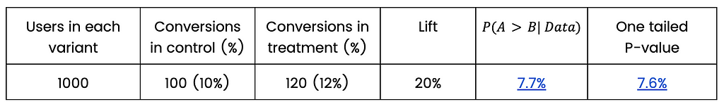
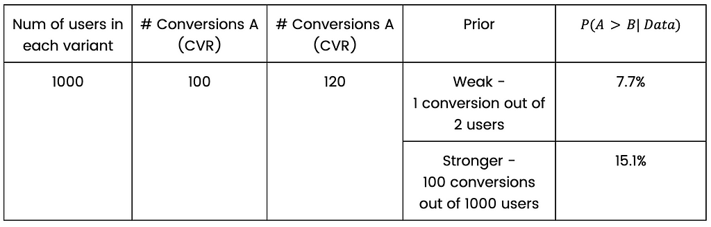
In the case of comparing two proportions — the meaning of prior is actually very simple. It is simply an addition of a virtual # of success and # of users to the data. Suppose we did such a test, and out of 1000 users in the control group, and we have 100 conversions.
Assuming my prior is “10 successes out of 100 users”, it means that my posterior knowledge is the sum of successes and users of the prior and the data. In our example: 110 “conversions” out of 1100 “users”. This is not the exact statistical definition, but it captures the idea very well.
A prior can be weak (1 success out of 10 users) or strong (1000 successes out of 10000 users for example). Both represent a knowledge that the conversion rate is 10%. In any case, when we accumulate a lot of data, the prior weight naturally decreases.
How should we incorporate prior knowledge in a two proportions A/B test? There are two options:
We incorporate, based on historical data, the general conversion rate in the population and add it to each variant. This is common practice.
We incorporate, based on historical data, which variant, control or treatment, usually show better results and give that variant an advantage based on this knowledge.
How will the prior manifest in the first option? Let’s stick to the example of 1000 users in each variant, 100 conversions to control variant and 120 conversions to treatment variant.
Suppose we know that the CVR is 10%, so an appropriate prior could be to add 100 successes and 1000 users to the existing data and then perform a statistical test as if we have 2000 users in each group, 200 conversions in control and 220 conversions in treatment. What’s described here is exactly what happens; it’s not approximately or as if — that’s the technical meaning of the prior in the case of two proportions bayesian test (assuming beta prior, for the statisticians reading this article).
A simple calculation shows that using a stronger prior in our example will increase P(A>B| Data), which means less indication for difference between variants — compared to the weak prior. That is what happens when you add the same amount of successes and users to each variant. This practice goes against our motivation to stop as early as possible, so why on earth would we want to do such a thing?
A common argument is that the Bayesian method is very liberal in choosing a winner, and the priors are a restraining factor. That’s true, the Bayesian method as I represented is very liberal, and priors are a restraining factor. So why not choose a more conservative approach (hmmm hmmm Frequentist) to begin with?
Moreover, if that is the argument, then it is clear to everyone that the glorified claim about priors that “add business information to the experiment” is misleading. If the business information is just a restraining factor, then the idea of using strong prior does not seem appealing at all.
The second option for incorporating a prior, giving one version an advantage over the other version based on historical data, is even worse. Why would anyone want to do this? Why should one experiment be influenced by the successes or failures of previous experiments? Each experiment should be a clean slate, a new opportunity to try something new without bias. Adding 200 successes to one version and 100 to the other sounds absurd and unreasonable in any way.
Language and Terminology
The third argument in favor of Bayesian A/B testing is the more intuitive language and terminology. A/B testing results are often consumed by people without strong statistical backgrounds. Frequentist metrics like p-values and confidence intervals can be unintuitive and misunderstood, even by statisticians. Many articles have been written about people’s misunderstanding of these metrics, even people with a background in statistics. I admit that it was only a considerable time after my master’s degree in statistics that I understood the exact definition of a classical CI. There is no doubt that this is a real pain point and an important one.
If you ask someone without a background in statistics to compare two versions with partial performance data for each version and ask them to formulate a question, they are likely to ask, “What is the probability that this version is better than the other version?” The same is true for confidence intervals. Most likely, when you explain the definition of a Frequentist confidence interval to someone, they will understand it in a Bayesian way.
This argument is actually true. I agree that Bayesian statistical metrics are much more intuitive to the common practitioner, and I agree that it is preferred that the statistical language will be as simple as possible and well understood, since A/B testing is mostly being conducted and consumed by non-statisticians. However, I don’t think it’s a disaster that practitioners don’t fully understand the statistical terms and results. Most of them are thinking in terms of “winning” and “losing” and it’s okay.
I recall, when I was at Wix, showing our new Bayesian A/B testing dashboard to a product manager as part of a usability test, to learn how he reads it and what he understands. His approach was very simple — searching for “greens” and “reds” KPIs and ignoring the “grays” KPIs. He didn’t really care if it was a p-value or probability B is better than A, a confidence interval or a credible interval. I bet that if he knew, it would rarely change his decision about the test.
Major Drawbacks of the Bayesian Method
So far, we have discussed the alleged advantages of using the popular Bayesian method for A/B testing and why some of them are not correct or meaningful enough. There are also very considerable disadvantages to using the Bayesian method:
The lack of maximum sample size
The lack of guidelines and framework to make a decision regarding the test when the results are inconclusive.
These drawbacks are significant, especially since most experiments do not show a significant effect.
Let’s assume we run an experiment which does not affect the KPI we are interested in at all. In most cases, the data will indicate indecision, and we will not be sure what to do next. Should we continue the experiment and collect more data? Or go with the more probable variant even if the results are not conclusive?
One can argue that predefined sample size is a limiting factor, but it also provides an important framework for decision-making. We decide upon a sample size, and we know that we will be able, with high probability (known as statistical power), detect a predefined effect size. If we are smart enough, we will use a sequential testing method that will allow us to stop before we reach the maximum predefined sample size.
It is true that when using one of the Bayesian stopping rules mentioned before, the test will eventually end even if there is no effect. For example, the risk will gradually, and slowly, decrease and eventually will reach the predefined threshold. The problem is it will take a very long time when there is no difference between the variants. So long that in reality practitioners will likely won’t have the patience to wait. They will stop the experiment once they feel there is no point in continuing.
When to Use Bayesian Methods in Experiments
In Multi-Armed Bandit (MAB) experiments, Bayesian statistics flourish and are considered best practice. In these types of experiments, there are usually several variants (for example several ads creative) and we want to quickly decide which ads are performing the best. When the experiment begins, users are allocated equally to all variants, but after some data is gathered, the allocation changes and more users are allocated to the better performing variant (ad). Eventually, (almost) all users are allocated to the best performing variant (ad).
I also came across an interesting Bayesian A/B testing framework in an article published by Microsoft, but I never met any organization using the suggested methodology, and it still lacks a maximum sample size which should be very important to practitioners.
Conclusion
While Bayesian A/B testing offers a more intuitive framework and the ability to incorporate prior knowledge, it falls short in critical areas. The promises of early stopping and better decision-making are not inherently guaranteed by Bayesian methods and can lead to misunderstandings and inflated false positive rates if not carefully managed. Additionally, the use of priors can introduce bias and complicate results rather than clarify them. The Frequentist approach, with its structured methodology and sequential testing options, provides more reliable and transparent results, especially in environments where rigorous decision-making is essential.
Let’s say you are in a customer care center, and you would like to know the probability distribution of the number of calls per minute, or in other words, you want to answer the question: what is the probability of receiving zero, one, two, … etc., calls per minute? You need this distribution in order to predict the probability of receiving different number of calls based on which you can plan how many employees are needed, whether or not an expansion is required, etc.
In order to let our decision ‘data informed’ we start by collecting data from which we try to infer this distribution, or in other words, we want to generalize from the sample data to the unseen data which is also known as the population in statistical terms. This is the essence of statistical inference.
From the collected data we can compute the relative frequency of each value of calls per minute. For example, if the collected data over time looks something like this: 2, 2, 3, 5, 4, 5, 5, 3, 6, 3, 4, … etc. This data is obtained by counting the number of calls received every minute. In order to compute the relative frequency of each value you can count the number of occurrences of each value divided by the total number of occurrences. This way you will end up with something like the grey curve in the below figure, which is equivalent to the histogram of the data in this example.
Image generated by the Author
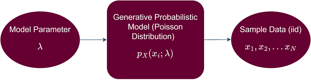
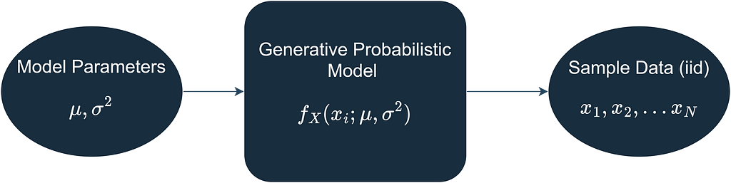
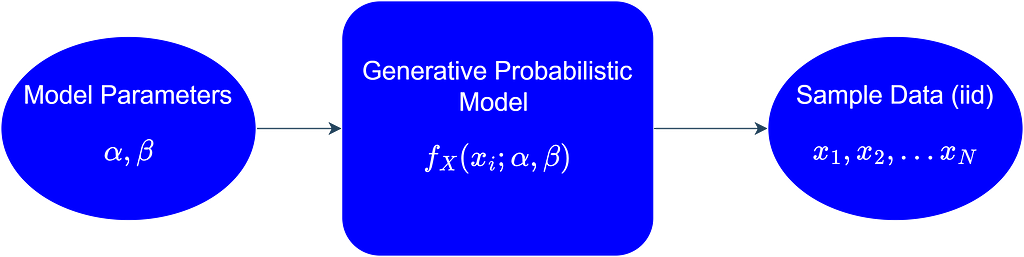
Another option is to assume that each data point from our data is a realization of a random variable (X) that follows a certain probability distribution. This probability distribution represents all the possible values that are generated if we were to collect this data long into the future, or in other words, we can say that it represents the population from which our sample data was collected. Furthermore, we can assume that all the data points come from the same probability distribution, i.e., the data points are identically distributed. Moreover, we assume that the data points are independent, i.e., the value of one data point in the sample is not affected by the values of the other data points. The independence and identical distribution (iid) assumption of the sample data points allows us to proceed mathematically with our statistical inference problem in a systematic and straightforward way. In more formal terms, we assume that a generative probabilistic model is responsible for generating the iid data as shown below.
Image generated by the Author
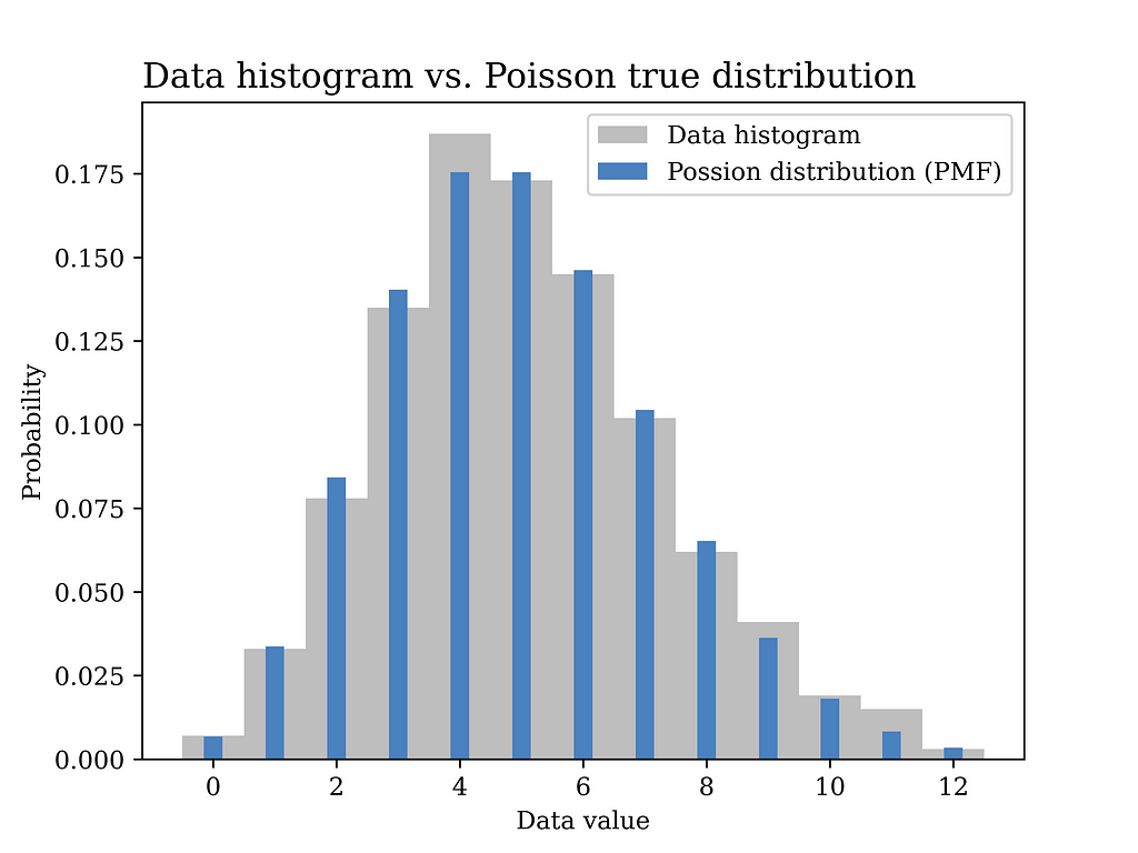
In this particular example, a Poisson distribution with mean value λ = 5 is assumed to have generated the data as shown in the blue curve in the below figure. In other words, we assume here that we know the true value of λ which is generally not known and needs to be estimated from the data.
Image generated by the Author
As opposed to the previous method in which we had to compute the relative frequency of each value of calls per minute (e.g., 12 values to be estimated in this example as shown in the grey figure above), now we only have one parameter that we aim at finding which is λ. Another advantage of this generative model approach is that it is better in terms of generalization from sample to population. The assumed probability distribution can be said to have summarized the data in an elegant way that follows the Occam’s razor principle.
Before proceeding further into how we aim at finding this parameter λ, let’s show some Python code first that was used to generate the above figure.
# Import the Python libraries that we will need in this article import pandas as pd import matplotlib.pyplot as plt import numpy as np import seaborn as sns import math from scipy import stats
# Poisson distribution example lambda_ = 5 sample_size = 1000 data_poisson = stats.poisson.rvs(lambda_,size= sample_size) # generate data
# Plot the data histogram vs the PMF x1 = np.arange(data_poisson.min(), data_poisson.max(), 1) fig1, ax = plt.subplots() plt.bar(x1, stats.poisson.pmf(x1,lambda_), label="Possion distribution (PMF)",color = BLUE2,linewidth=3.0,width=0.3,zorder=2) ax.hist(data_poisson, bins=x1.size, density=True, label="Data histogram",color = GRAY9, width=1,zorder=1,align='left')
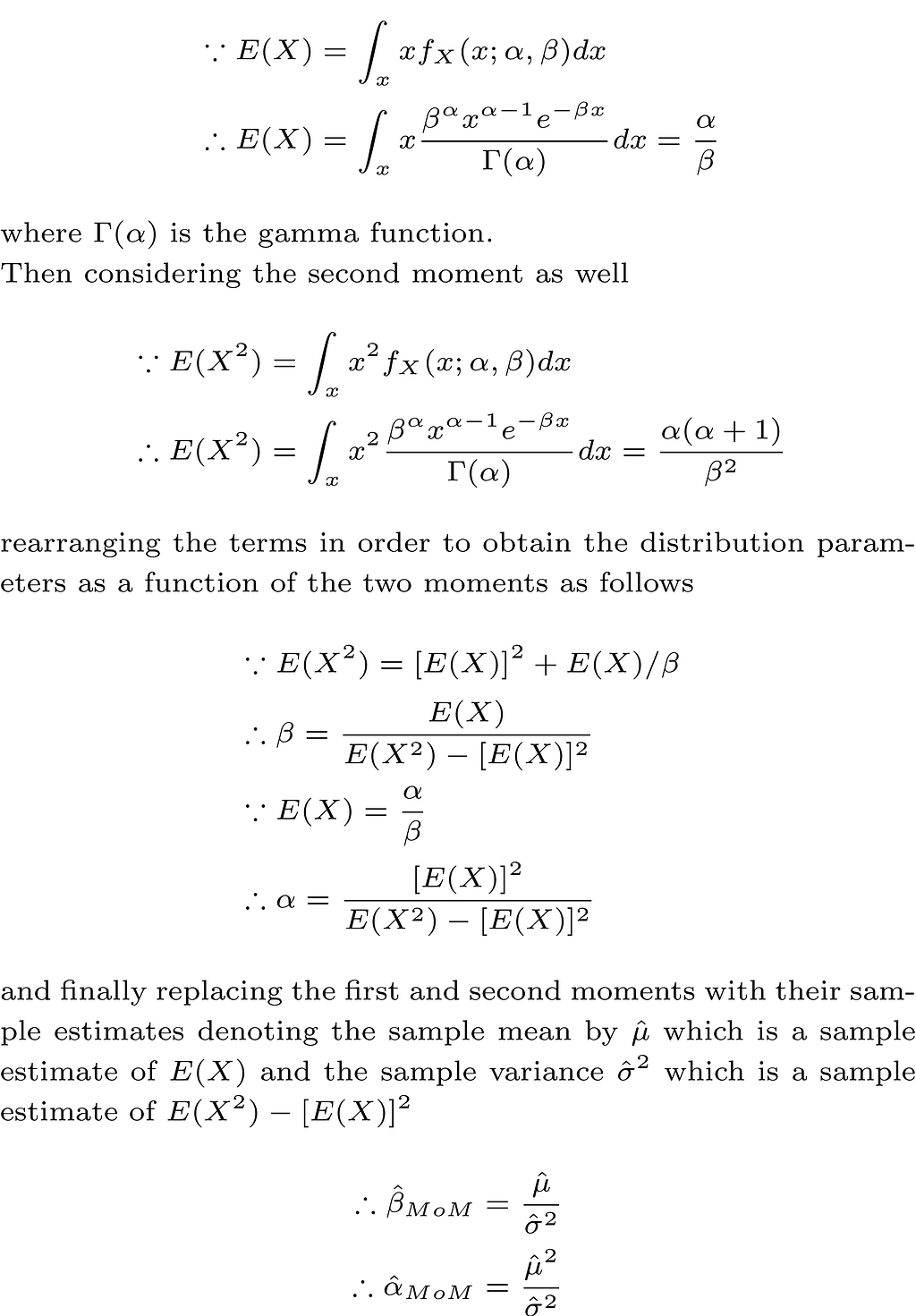
Our problem now is about estimating the value of the unknown parameter λ using the data we collected. This is where we will use the method of moments (MoM) approach that appears in the title of this article.
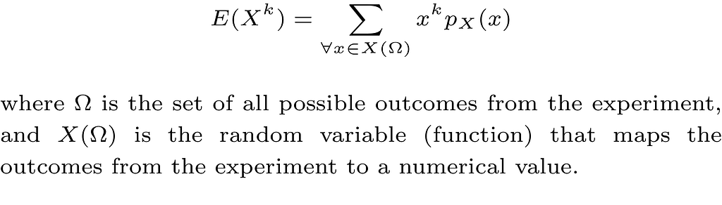
First, we need to define what is meant by the moment of a random variable. Mathematically, the kth moment of a discrete random variable (X) is defined as follows
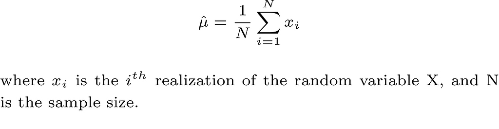
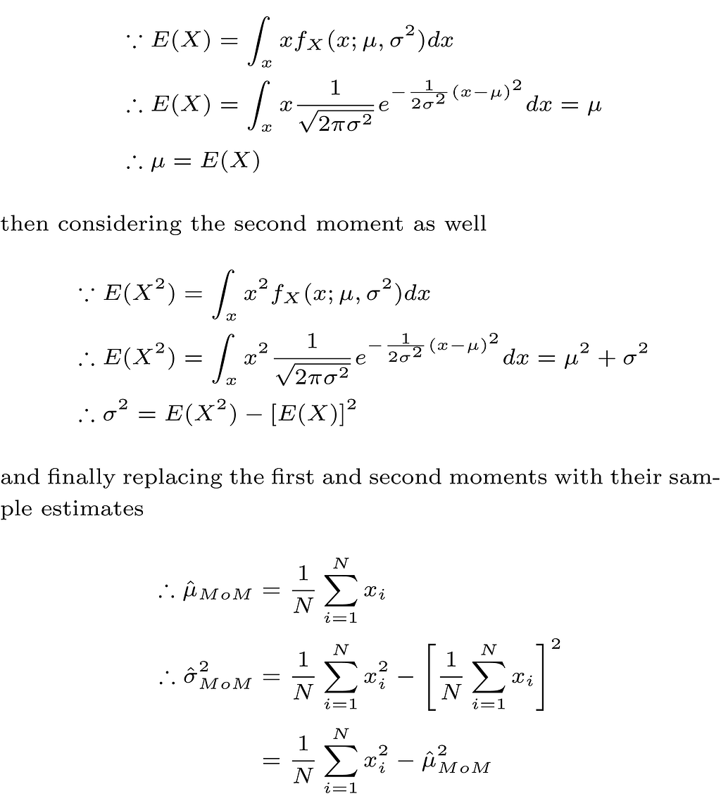
Take the first moment E(X) as an example, which is also the mean μ of the random variable, and assuming that we collect our data which is modeled as N iid realizations of the random variable X. A reasonable estimate of μ is the sample mean which is defined as follows
Thus, in order to obtain a MoM estimate of a model parameter that parametrizes the probability distribution of the random variable X, we first write the unknown parameter as a function of one or more of the kth moments of the random variable, then we replace the kth moment with its sample estimate. The more unknown parameters we have in our models, the more moments we need.
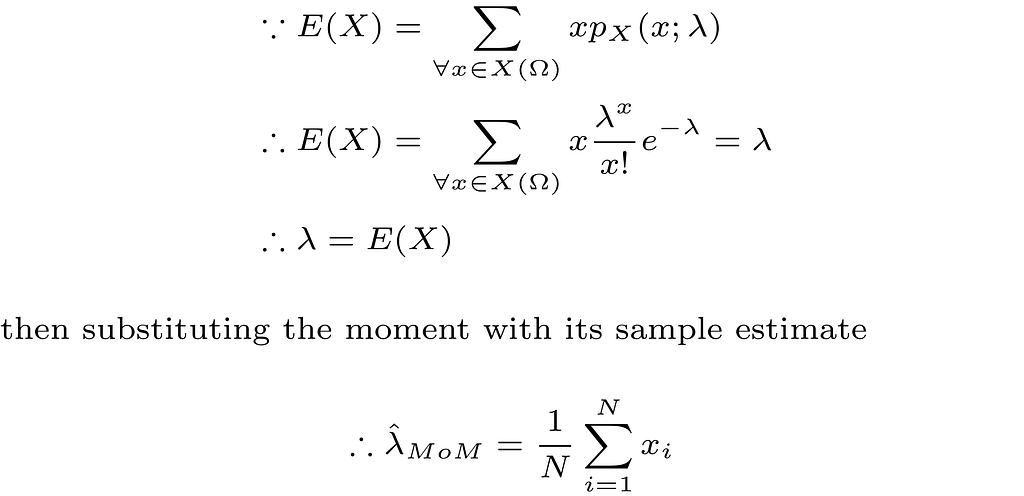
In our Poisson model example, this is very simple as shown below
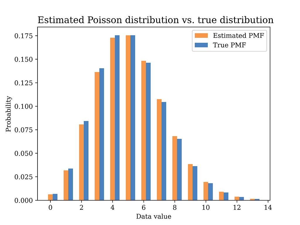
In the next part, we test our MoM estimator on the simulated data we had earlier. The Python code for obtaining the estimator and plotting the corresponding probability distribution using the estimated parameter is shown below.
# Method of moments estimator using the data (Poisson Dist) lambda_hat = sum(data_poisson) / len(data_poisson)
ax.set_title("Estimated Poisson distribution vs. true distribution", fontsize=14, loc='left') ax.set_xlabel('Data value') ax.set_ylabel('Probability') ax.legend() #ax.grid() plt.savefig("Possion_true_vs_est.png", format="png", dpi=800)
The below figure shows the estimated distribution versus the true distribution. The distributions are quite close indicating that the MoM estimator is a reasonable estimator for our problem. In fact, replacing expectations with averages in the MoM estimator implies that the estimator is a consistent estimator by the law of large numbers, which is a good justification for using such estimator.
Image generated by the Author
Another MoM estimation example is shown below assuming the iid data is generated by a normal distribution with mean μ and variance σ² as shown below.
Image generated by the Author
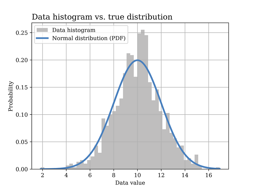
In this particular example, a Gaussian (normal) distribution with mean value μ = 10 and σ = 2 is assumed to have generated the data. The histogram of the generated data sample (sample size = 1000) is shown in grey in the below figure, while the true distribution is shown in the blue curve.
Image generated by the Author
The Python code that was used to generate the above figure is shown below.
# Normal distribution example mu = 10 sigma = 2 sample_size = 1000 data_normal = stats.norm.rvs(loc=mu, scale=sigma ,size= sample_size) # generate data
# Plot the data histogram vs the PDF x2 = np.linspace(data_normal.min(), data_normal.max(), sample_size) fig3, ax = plt.subplots() ax.hist(data_normal, bins=50, density=True, label="Data histogram",color = GRAY9) ax.plot(x2, stats.norm(loc=mu, scale=sigma).pdf(x2), label="Normal distribution (PDF)",color = BLUE2,linewidth=3.0)
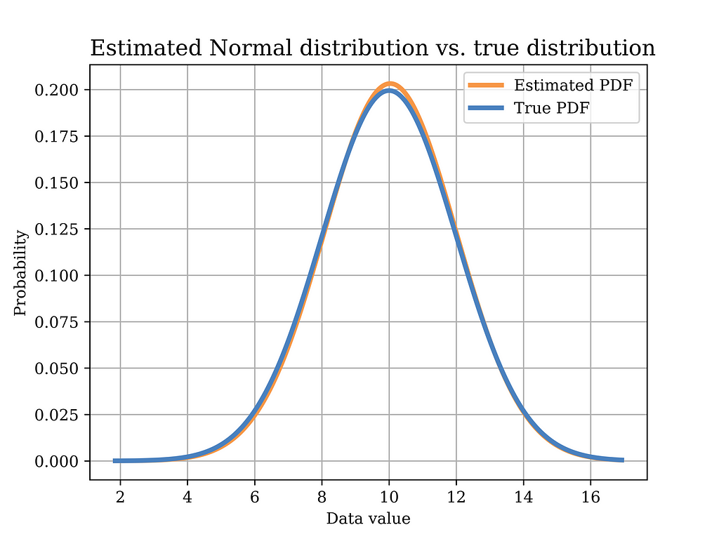
Now, we would like to use the MoM estimator to find an estimate of the model parameters, i.e., μ and σ² as shown below.
In order to test this estimator using our sample data, we plot the distribution with the estimated parameters (orange) in the below figure, versus the true distribution (blue). Again, it can be shown that the distributions are quite close. Of course, in order to quantify this estimator, we need to test it on multiple realizations of the data and observe properties such as bias, variance, etc. Such important aspects have been discussed in an earlier article Bias Variance Tradeoff in Parameter Estimation with Python Code | by Mahmoud Abdelaziz, PhD | Medium
Image generated by the Author
The Python code that was used to estimate the model parameters using MoM, and to plot the above figure is shown below.
# Method of moments estimator using the data (Normal Dist)
mu_hat = sum(data_normal) / len(data_normal) # MoM mean estimator
var_hat = sum(pow(x-mu_hat,2) for x in data_normal) / len(data_normal) # variance
sigma_hat = math.sqrt(var_hat)  # MoM standard deviation estimator

# Plot the MoM estimated PDF vs the true PDF
x2 = np.linspace(data_normal.min(), data_normal.max(), sample_size)
fig4, ax = plt.subplots()
ax.plot(x2, stats.norm(loc=mu_hat, scale=sigma_hat).pdf(x2),
        label="Estimated PDF",color = ORANGE1,linewidth=3.0)
ax.plot(x2, stats.norm(loc=mu, scale=sigma).pdf(x2),
        label="True PDF",color = BLUE2,linewidth=3.0)

ax.set_title("Estimated Normal distribution vs. true distribution", fontsize=14, loc='left')
ax.set_xlabel('Data value')
ax.set_ylabel('Probability')
ax.legend()
ax.grid()
plt.savefig("Normal_true_vs_est.png", format="png", dpi=800)
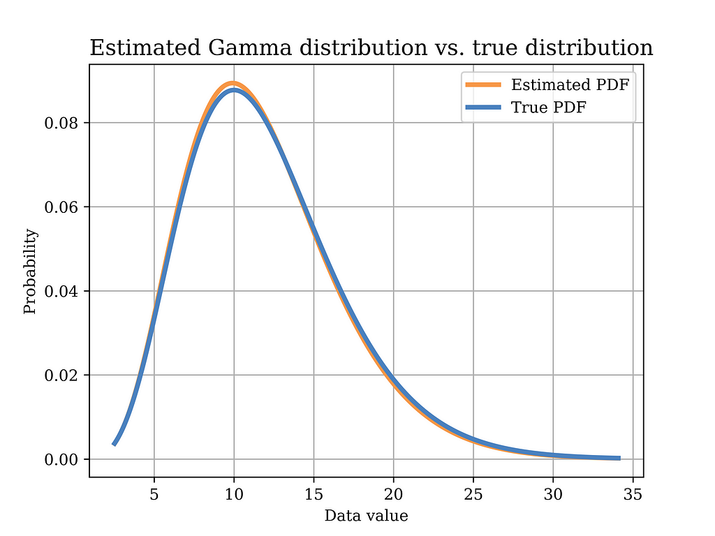
Another useful probability distribution is the Gamma distribution. An example for the application of this distribution in real life was discussed in a previous article. However, in this article, we derive the MoM estimator of the Gamma distribution parameters α and β as shown below, assuming the data is iid.
Image generated by the Author
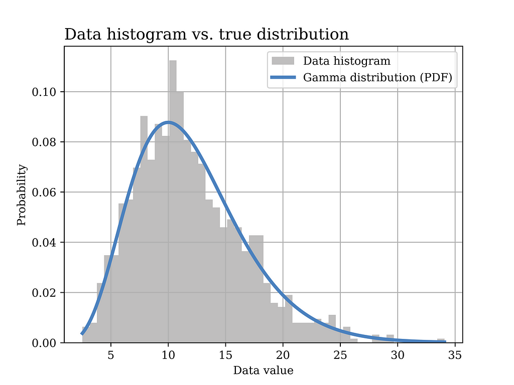
In this particular example, a Gamma distribution with α = 6 and β = 0.5 is assumed to have generated the data. The histogram of the generated data sample (sample size = 1000) is shown in grey in the below figure, while the true distribution is shown in the blue curve.
Image generated by the Author
The Python code that was used to generate the above figure is shown below.
# Gamma distribution example alpha_ = 6 # shape parameter scale_ = 2 # scale paramter (lamda) = 1/beta in gamma dist. sample_size = 1000 data_gamma = stats.gamma.rvs(alpha_,loc=0, scale=scale_ ,size= sample_size) # generate data
# Plot the data histogram vs the PDF x3 = np.linspace(data_gamma.min(), data_gamma.max(), sample_size) fig5, ax = plt.subplots() ax.hist(data_gamma, bins=50, density=True, label="Data histogram",color = GRAY9) ax.plot(x3, stats.gamma(alpha_,loc=0, scale=scale_).pdf(x3), label="Gamma distribution (PDF)",color = BLUE2,linewidth=3.0)
Now, we would like to use the MoM estimator to find an estimate of the model parameters, i.e., α and β, as shown below.
In order to test this estimator using our sample data, we plot the distribution with the estimated parameters (orange) in the below figure, versus the true distribution (blue). Again, it can be shown that the distributions are quite close.
Image generated by the Author
The Python code that was used to estimate the model parameters using MoM, and to plot the above figure is shown below.
# Method of moments estimator using the data (Gamma Dist) sample_mean = data_gamma.mean() sample_var = data_gamma.var() scale_hat = sample_var/sample_mean #scale is equal to 1/beta in gamma dist. alpha_hat = sample_mean**2/sample_var
# Plot the MoM estimated PDF vs the true PDF x4 = np.linspace(data_gamma.min(), data_gamma.max(), sample_size) fig6, ax = plt.subplots()
ax.set_title("Estimated Gamma distribution vs. true distribution", fontsize=14, loc='left') ax.set_xlabel('Data value') ax.set_ylabel('Probability') ax.legend() ax.grid() plt.savefig("Gamma_true_vs_est.png", format="png", dpi=800)
Note that we used the following equivalent ways of writing the variance when deriving the estimators in the cases of Gaussian and Gamma distributions.
Conclusion
In this article, we explored various examples of the method of moments estimator and its applications in different problems in data science. Moreover, detailed Python code that was used to implement the estimators from scratch as well as to plot the different figures is also shown. I hope that you will find this article helpful.
Rebellion’s award-winning tactical shooter, “Sniper Elite 4” is now available on select iPhone, iPad, and Mac devices.
Sniper Elite 4 | Image Credit: Rebellion
The World War II sniper experience takes the player to 1943 Italy. Playing as Karl Fairburne, they must use an array of authentic weaponry to defeat a new Nazi threat.
The game is best known for its “X-ray Kill Camera,” which shows an internal view of enemies as they are hit by bullets.
The Screen Actors Guild has announced its award nominations for 2025, with Apple TV+ getting all of its nods for the thriller “Slow Horses,” and the comedy “Shrinking.”
Gary Oldman in “Slow Horses” — image credit: Apple TV+
In 2024, Apple TV+ scored 11 SAG-AFTRA nominations, led chiefly by “Ted Lasso.” For the new 31st Screen Actors Guild Awards, it’s received four nominations, all for just two shows.
Gary Oldman is nominated as Outstanding Performance by a Male Actor in a Drama Series for his role in “Slow Horses.” He’s competing against Eddie Redmayne for Sky/Universal’s “The Day of the Jackal,” Jeff Bridges for FX’s “The Old Man,” and both Tadanobu Asano and Hiroyuki Sanada for “Shogun.”
Apple TV+ hits ‘Slow Horses’ and ‘Shrinking’ nominated for acting awards
Originally appeared here:
Apple TV+ hits ‘Slow Horses’ and ‘Shrinking’ nominated for acting awards
We use cookies on our website to give you the most relevant experience by remembering your preferences and repeat visits. By clicking “Accept”, you consent to the use of ALL the cookies.
This website uses cookies to improve your experience while you navigate through the website. Out of these, the cookies that are categorized as necessary are stored on your browser as they are essential for the working of basic functionalities of the website. We also use third-party cookies that help us analyze and understand how you use this website. These cookies will be stored in your browser only with your consent. You also have the option to opt-out of these cookies. But opting out of some of these cookies may affect your browsing experience.
Necessary cookies are absolutely essential for the website to function properly. These cookies ensure basic functionalities and security features of the website, anonymously.
Cookie
Duration
Description
cookielawinfo-checkbox-analytics
11 months
This cookie is set by GDPR Cookie Consent plugin. The cookie is used to store the user consent for the cookies in the category "Analytics".
cookielawinfo-checkbox-functional
11 months
The cookie is set by GDPR cookie consent to record the user consent for the cookies in the category "Functional".
cookielawinfo-checkbox-necessary
11 months
This cookie is set by GDPR Cookie Consent plugin. The cookies is used to store the user consent for the cookies in the category "Necessary".
cookielawinfo-checkbox-others
11 months
This cookie is set by GDPR Cookie Consent plugin. The cookie is used to store the user consent for the cookies in the category "Other.
cookielawinfo-checkbox-performance
11 months
This cookie is set by GDPR Cookie Consent plugin. The cookie is used to store the user consent for the cookies in the category "Performance".
viewed_cookie_policy
11 months
The cookie is set by the GDPR Cookie Consent plugin and is used to store whether or not user has consented to the use of cookies. It does not store any personal data.
Functional cookies help to perform certain functionalities like sharing the content of the website on social media platforms, collect feedbacks, and other third-party features.
Performance cookies are used to understand and analyze the key performance indexes of the website which helps in delivering a better user experience for the visitors.
Analytical cookies are used to understand how visitors interact with the website. These cookies help provide information on metrics the number of visitors, bounce rate, traffic source, etc.
Advertisement cookies are used to provide visitors with relevant ads and marketing campaigns. These cookies track visitors across websites and collect information to provide customized ads.