A comprehensive guide on getting the most out of your Chinese topic models, from preprocessing to interpretation.
With our recent paper on discourse dynamics in European Chinese diaspora media, our team has tapped into an almost unanimous frustration with the quality of topic modelling approaches when applied to Chinese data. In this article, I will introduce you to our novel topic modelling method, KeyNMF, and how to apply it most effectively to Chinese textual data.
Topic Modelling with Matrix Factorization
Before diving into practicalities, I would like to give you a brief introduction to topic modelling theory, and motivate the advancements introduced in our paper.
Topic modelling is a discipline of Natural Language Processing for uncovering latent topical information in textual corpora in an unsupervised manner, that is then presented to the user in a human-interpretable way (usually 10 keywords for each topic).
There are many ways to formalize this task in mathematical terms, but one rather popular conceptualization of topic discovery is matrix factorization. This is a rather natural and intuitive way to tackle the problem, and in a minute, you will see why. The primary insight behind topic modelling as matrix factorization is the following: Words that frequently occur together, are likely to belong to the same latent structure. In other words: Terms, the occurrence of which are highly correlated, are part of the same topic.
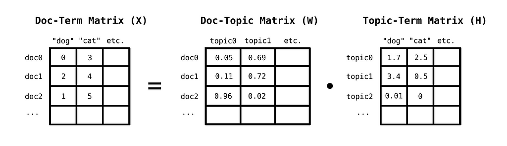
You can discover topics in a corpus, by first constructing a bag-of-words matrix of documents. A bag-of-words matrix represents documents in the following way: Each row corresponds to a document, while each column to a unique word from the model’s vocabulary. The values in the matrix are then the number of times a word occurs in a given document.
Schematic Overview of Non-negative Matrix Factorization
This matrix can be decomposed into the linear combination of a topic-term matrix, which indicates how important a word is for a given topic,and a document-topic matrix, which indicates how important a given topic is for a given document. A method for this decomposition is Non-negative Matrix Factorization, where we decompose a non-negative matrix to two other strictly non-negative matrices, instead of allowing arbitrary signed values.
NMF is not the only method one can use for decomposing the bag-of-words matrix. A method of high historical significance, Latent Semantic Analysis, utilizes Truncated Singular-Value Decomposition for this purpose. NMF, however, is generally a better choice, as:
The discovered latent factors are of different quality from other decomposition methods. NMF typically discovers localized patterns or parts in the data, which are easier to interpret.
Non-negative topic-term and document-topic relations are easier to interpret than signed ones.
Using NMF with just BoW matrices, however attractive and simple it may be, does come with its setbacks:
NMF typically minimizes the Frobenius norm of the error matrix. This entails an assumption of Gaussianity of the outcome variable, which is obviously false, as we are modelling word counts.
BoW representations are just word counts. This means that words won’t be interpreted in context, and syntactical information will be ignored.
KeyNMF
To account for these limitations, and with the help of new transformer-based language representations, we can significantly improve NMF for our purposes.
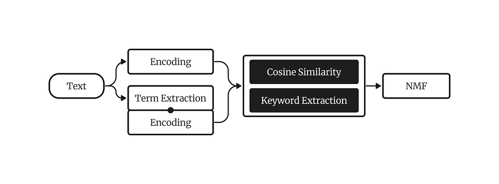
The key intuition behind KeyNMF is that most words in a document are semantically insignificant, and we can get an overview of topical information in the document by highlighting the top N most relevant terms. We will select these terms by using contextual embeddings from sentence-transformer models.
A Schematic Overview of the KeyNMF Model
The KeyNMF algorithm consists of the following steps:
Embed each document using a sentence-transformer, along with all words in the document.
Calculate cosine similarities of word embeddings to document embeddings.
For each document, keep the highest N words with positive cosine similarities to the document.
Arrange cosine similarities into a keyword-matrix, where each row is a document, each column is a keyword, and values are cosine similarities of the word to the document.
Decompose the keyword matrix with NMF.
This formulation helps us in multiple ways. a) We substantially reduce the model’s vocabulary, thereby having less parameters, resulting in faster and better model fit b) We get continuous distribution, which is a better fit for NMF’s assumptions and c) We incorporate contextual information into our topic model.
Chinese Topic Modelling with KeyNMF
Now that you understand how KeyNMF works, let’s get our hands dirty and apply the model in a practical context.
Preparation and Data
First, let’s install the packages we are going to use in this demonstration:
Then let’s get some openly available data. I chose to go with the SIB200 corpus, as it is freely available under the CC-BY-SA 4.0 open license. This piece of code will fetch us the corpus.
from datasets import load_dataset

# Loads the dataset
ds = load_dataset("Davlan/sib200", "zho_Hans", split="all")
corpus = ds["text"]
Building a Chinese Topic Model
There are a number of tricky aspects to applying language models to Chinese, since most of these systems are developed and tested on English data. When it comes to KeyNMF, there are two aspects that need to be taken into account.
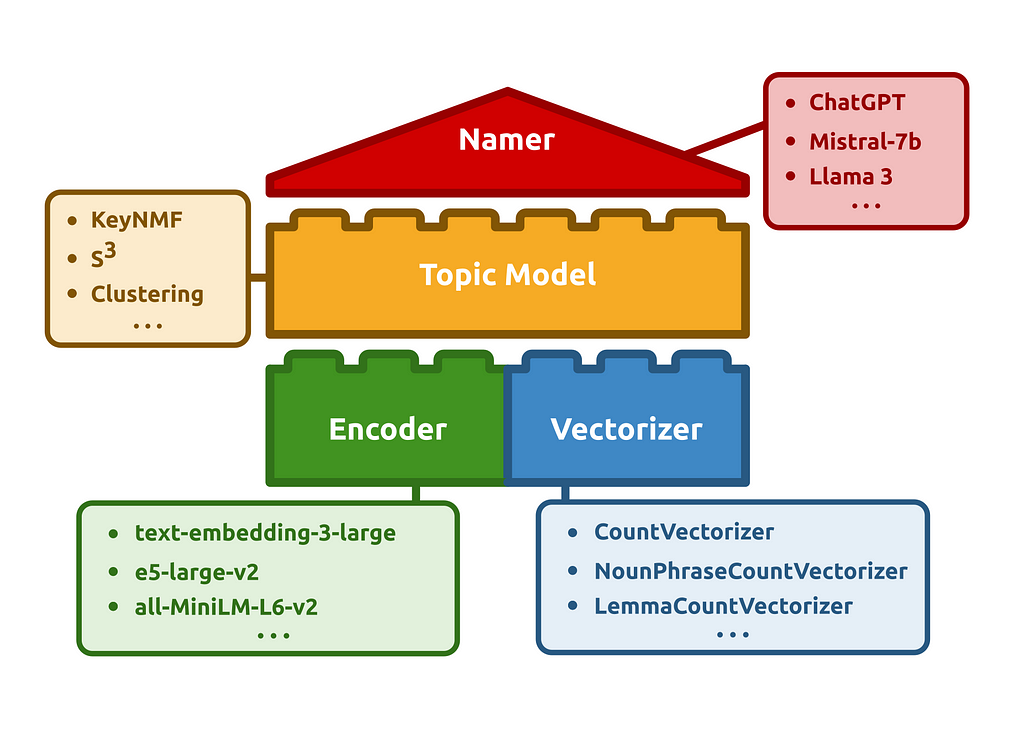
Elements of a Topic Modelling Pipeline in Turftopic
Firstly, we will need to figure out how to tokenize texts in Chinese. Luckily, the Turftopic library, which contains our implementation of KeyNMF (among other things), comes prepackaged with tokenization utilities for Chinese. Normally, you would use a CountVectorizer object from sklearn to extract words from text. We added a ChineseCountVectorizer object that uses the Jieba tokenizer in the background, and has an optionally usable Chinese stop word list.
from turftopic.vectorizers.chinese import ChineseCountVectorizer
Then we will need a Chinese embedding model for producing document and word representations. We will use the paraphrase-multilingual-MiniLM-L12-v2 model for this, as it is quite compact and fast, and was specifically trained to be used in multilingual retrieval contexts.
from sentence_transformers import SentenceTransformer
We can then build a fully Chinese KeyNMF model! I will initialize a model with 20 topics and N=25 (a maximum of 15 keywords will be extracted for each document)
from turftopic import KeyNMF

model = KeyNMF(
    n_components=20,
    top_n=25,
    vectorizer=vectorizer,
    encoder=encoder,
    random_state=42, # Setting seed so that our results are reproducible
)
We can then fit the model to the corpus and see what results we get!
As you see, we’ve already gained a sensible overview of what there is in our corpus! You can see that the topics are quite distinct, with some of them being concerned with scientific topics, such as astronomy (8), chemistry (5) or animal behaviour (9), while others were oriented at leisure (e.g. 0, 1, 12), or politics (19, 11).
Visualization
To gain further aid in understanding the results, we can use the topicwizard library to visually investigate the topic model’s parameters.
Since topicwizard uses wordclouds, we will need to tell the library that it should be using a font that is compatible with Chinese. I took a font from the ChineseWordCloud repo, that we will download and then pass to topicwizard.
This will open the topicwizard web app in a notebook or in your browser, with which you can interactively investigate your topic model:
Investigating the relations of topic, documents and words in your corpus using topicwizard
Conclusion
In this article, we’ve looked at what KeyNMF is, how it works, what it’s motivated by and how it can be used to discover high-quality topics in Chinese text, as well as how to visualize and interpret your results. I hope this tutorial will prove useful to those who are looking to explore Chinese textual data.
For further information on the models, and how to improve your results, I encourage you to check out our Documentation. If you should have any questions or encounter issues, feel free to submit an issue on Github, or reach out in the comments :))
All figures presented in the article were produced by the author.
llama.cpp has revolutionized the space of LLM inference by the means of wide adoption and simplicity. It has enabled enterprises and individual developers to deploy LLMs on devices ranging from SBCs to multi-GPU clusters. Though working with llama.cpp has been made easy by its language bindings, working in C/C++ might be a viable choice for performance sensitive or resource constrained scenarios.
This tutorial aims to let readers have a detailed look on how LLM inference is performed using low-level functions coming directly from llama.cpp. We discuss the program flow, llama.cpp constructs and have a simple chat at the end.
The C++ code that we will write in this blog is also used in SmolChat, a native Android application that allows users to interact with LLMs/SLMs in the chat interface, completely on-device. Specifically, the LLMInference class we define ahead is used with the JNI binding to execute GGUF models.
llama.cpp is a C/C++ framework to infer machine learning models defined in the GGUF format on multiple execution backends. It started as a pure C/C++ implementation of the famous Llama series LLMs from Meta that can be inferred on Apple’s silicon, AVX/AVX-512, CUDA, and Arm Neon-based environments. It also includes a CLI-based tool llama-cli to run GGUF LLM models and llama-server to execute models via HTTP requests (OpenAI compatible server).
llama.cpp uses ggml, a low-level framework that provides primitive functions required by deep learning models and abstracts backend implementation details from the user. Georgi Gerganov is the creator of ggml and llama.cpp.
The repository’s README also lists wrappers built on top of llama.cpp in other programming languages. Popular tools like Ollama and LM Studio also use bindings over llama.cpp to enhance user friendliness. The project has no dependencies on other third-party libraries
How is llama.cpp different from PyTorch/TensorFlow?
llama.cpp has emphasis on inference of ML models from its inception, whereas PyTorch and TensorFlow are end-to-end solutions offering data processing, model training/validation, and efficient inference in one package.
PyTorch and TensorFlow also have their lightweight inference-only extensions namely ExecuTorch and TensorFlow Lite
Considering only the inference phase of a model, llama.cpp is lightweight in its implementation due to the absence of third-party dependencies and an extensive set of available operators or model formats to support. Also, as the name suggests, the project started as an efficient library to infer LLMs (the Llama model from Meta) and continues to support a wide range of open-source LLM architectures.
Analogy: If PyTorch/TensorFlow are luxurious, power-hungry cruise ships, llama.cpp is small, speedy motorboat. PyTorch/TF and llama.cpp have their own use-cases.
Setup
We start our implementation in a Linux-based environment (native or WSL) with cmake installed and the GNU/clang toolchain installed. We’ll compile llama.cpp from source and add it as a shared library to our executable chat program.
We create our project directory smol_chat with aexternals directory to store the cloned llama.cpp repository.
mkdir smol_chat
cd smol_chat

mkdir src
mkdir externals
touch CMakeLists.txt

cd externals
git clone --depth=1 https://github.com/ggerganov/llama.cpp
CMakeLists.txt is where we define our build, allowing CMake to compile our C/C++ code using the default toolchain (GNU/clang) by including headers and shared libraries from externals/llama.cpp.
We have now defined how our project should be built by CMake. Next, we create a header file LLMInference.h which declares a class containing high-level functions to interact with the LLM. llama.cpp provides a C-style API, thus embedding it within a class will help us abstract/hide the inner working details.
// container to store user/assistant messages in the chat std::vector<llama_chat_message> _messages; // stores the string generated after applying // the chat-template to all messages in `_messages` std::vector<char> _formattedMessages; // stores the tokens for the last query // appended to `_messages` std::vector<llama_token> _promptTokens; int _prevLen = 0;
// stores the complete response for the given query std::string _response = "";
The private members declared in the header above will be used in the implementation of the public member functions described in the further sections of the blog. Let us define each of these member functions in LLMInference.cpp .
llama_load_model_from_filereads the model from the file using llama_load_model internally and populates the llama_model instance using the given llama_model_params . The user can give the parameters, but we can get a pre-initialized default struct for it with llama_model_default_params .
llama_context represents the execution environment for the GGUF model loaded. The llama_new_context_with_model instantiates a new llama_context and prepares a backend for execution by either reading the llama_model_params or by automatically detecting the available backends. It also initializes the K-V cache, which is important in the decoding or inference step. A backend scheduler that manages computations across multiple backends is also initialized.
A llama_sampler determines how we sample/choose tokens from the probability distribution derived from the outputs (logits) of the model (specifically the decoder of the LLM). LLMs assign a probability to each token present in the vocabulary, representing the chances of the token appearing next in the sequence. The temperature and min-p that we are setting with llama_sampler_init_temp and llama_sampler_init_min_p are two parameters controlling the token sampling process.
There are multiple steps involved in the inference process that takes a text query from the user as input and returns the LLM’s response.
1. Applying the chat template to the queries
For an LLM, the incoming messages are classified as belonging to three roles, user , assistant and system . user and assistant messages given by the user and the LLM, respectively, whereas system denotes a system-wide prompt that is followed across the entire conversation. Each message consists of a role and content where content is the actual text and role is any one of the three roles.
<example>
The system prompt is the first message of the conversation. In our code, the messages are stored as a std::vector<llama_chat_message> named _messages where llama_chat_message is a llama.cpp struct with role and content attributes. We use the llama_chat_apply_template function from llama.cpp to apply the chat template stored in the GGUF file as metadata. We store the string or std::vector<char> obtained after applying the chat template in _formattedMessages .
2. Tokenization
Tokenization is the process of dividing a given text into smaller parts (tokens). We assign each part/token a unique integer ID, thus transforming the input text to a sequence of integers that form the input to the LLM. llama.cpp provides the common_tokenize or llama_tokenize functions to perform tokenization, where common_tokenize returns the sequence of tokens as a std::vector<llama_token> .
// create a llama_batch containing a single sequence // see llama_batch_init for more details _batch.token = _promptTokens.data(); _batch.n_tokens = _promptTokens.size(); }
In the code, we apply the chat template and perform tokenization in the LLMInference::startCompletion method and then create a llama_batch instance holding the final inputs for the model.
3. Decoding, Sampling and the KV Cache
As highlighted earlier, LLMs generate a response by successively predicting the next token in the given sequence. LLMs are also trained to predict a special end-of-generation (EOG) token, indicating the end of the sequence of the predicted tokens. The completion_loop function returns the next token in the sequence and keeps getting called until the token it returns is the EOG token.
Using llama_n_ctx and the llama_get_kv_cached_used_cells we determine the length of the context we have utilized for storing the inputs. Currently, we throw an error if the length of the tokenized inputs exceeds the context size.
llama_decode performs a forward-pass of the model, given the inputs in _batch .
Using the _sampler initialized in the LLMInference::loadModel we sample or choose a token as our prediction and store it in _currToken . We check if the token is an EOG token and then return an “EOG” indicating that the text generation loop calling LLMInference::completionLoop should be terminated. On termination, we append a new message to _messages which is the complete _response given by the LLM with role assistant .
_currToken is still an integer, which is converted to a string token piece by the common_token_to_piece function. This string token is returned from the completionLoop method.
We need to reinitialize _batch to ensure it now only contains _currToken and not the entire input sequence, i.e. _promptTokens . This is because the ‘keys’ and ‘values’ for all previous tokens have been cached. This reduces the inference time by avoiding the computation of all ‘keys’ and ‘values’ for all tokens in _promptTokens .
std::string LLMInference::completionLoop() {
    // check if the length of the inputs to the model
    // have exceeded the context size of the model
    int contextSize = llama_n_ctx(_ctx);
    int nCtxUsed = llama_get_kv_cache_used_cells(_ctx);
    if (nCtxUsed + _batch.n_tokens > contextSize) {
        std::cerr << "context size exceeded" << 'n';
        exit(0);
    }
    // run the model
    if (llama_decode(_ctx, _batch) < 0) {
        throw std::runtime_error("llama_decode() failed");
    }

    // sample a token and check if it is an EOG (end of generation token)
    // convert the integer token to its corresponding word-piece
    _currToken = llama_sampler_sample(_sampler, _ctx, -1);
    if (llama_token_is_eog(_model, _currToken)) {
        addChatMessage(strdup(_response.data()), "assistant");
        _response.clear();
        return "[EOG]";
    }
    std::string piece = common_token_to_piece(_ctx, _currToken, true);


    // re-init the batch with the newly predicted token
    // key, value pairs of all previous tokens have been cached
    // in the KV cache
    _batch.token = &_currToken;
    _batch.n_tokens = 1;

    return piece;
}
Also, for each query made by the user, LLM takes as input the entire tokenized conversation (all messages stored in _messages ). If we tokenize the entire conversation every time in the startCompletion method, the preprocessing time and thus the overall inference time will increase as the conversation gets longer.
To avoid this computation, we only need to tokenize the latest message/query added to _messages . The length up to which messages in _formattedMessages have been tokenized is stored in _prevLen . At the end of response generation, i.e. in LLMInference::stopCompletion , we update the value of _prevLen , by appending the LLM’s response to _messages and using the return value of llama_chat_apply_template .
We implement a destructor method that deallocates dynamically-allocated objects, both in _messages and llama. cpp internally.
LLMInference::~LLMInference() {
    // free memory held by the message text in messages
    // (as we had used strdup() to create a malloc'ed copy)
    for (llama_chat_message &message: _messages) {
        delete message.content;
    }
    llama_kv_cache_clear(_ctx);
    llama_sampler_free(_sampler);
    llama_free(_ctx);
    llama_free_model(_model);
}
Writing a Small CMD Application
We create a small interface that allows us to have a conversion with the LLM. This includes instantiating the LLMInference class and calling all methods that we defined in the previous sections.
We use the CMakeLists.txt authored in one of the previous sections that use it to create a Makefile which will compile the code and create an executable ready for use.
mkdir build
cd build
cmake ..
make
./chat
Here’s how the output looks:
register_backend: registered backend CPU (1 devices)
register_device: registered device CPU (11th Gen Intel(R) Core(TM) i3-1115G4 @ 3.00GHz)
llama_model_loader: loaded meta data with 33 key-value pairs and 290 tensors from /home/shubham/CPP_Projects/llama-cpp-inference/models/smollm2-360m-instruct-q8_0.gguf (version GGUF V3 (latest))
llama_model_loader: Dumping metadata keys/values. Note: KV overrides do not apply in this output.
llama_model_loader: - kv   0:                       general.architecture str              = llama
llama_model_loader: - kv   1:                               general.type str              = model
llama_model_loader: - kv   2:                               general.name str              = Smollm2 360M 8k Lc100K Mix1 Ep2
llama_model_loader: - kv   3:                       general.organization str              = Loubnabnl
llama_model_loader: - kv   4:                           general.finetune str              = 8k-lc100k-mix1-ep2
llama_model_loader: - kv   5:                           general.basename str              = smollm2
llama_model_loader: - kv   6:                         general.size_label str              = 360M
llama_model_loader: - kv   7:                            general.license str              = apache-2.0
llama_model_loader: - kv   8:                          general.languages arr[str,1]       = ["en"]
llama_model_loader: - kv   9:                          llama.block_count u32              = 32
llama_model_loader: - kv  10:                       llama.context_length u32              = 8192
llama_model_loader: - kv  11:                     llama.embedding_length u32              = 960
llama_model_loader: - kv  12:                  llama.feed_forward_length u32              = 2560
llama_model_loader: - kv  13:                 llama.attention.head_count u32              = 15
llama_model_loader: - kv  14:              llama.attention.head_count_kv u32              = 5
llama_model_loader: - kv  15:                       llama.rope.freq_base f32              = 100000.000000
llama_model_loader: - kv  16:     llama.attention.layer_norm_rms_epsilon f32              = 0.000010
llama_model_loader: - kv  17:                          general.file_type u32              = 7
llama_model_loader: - kv  18:                           llama.vocab_size u32              = 49152
llama_model_loader: - kv  19:                 llama.rope.dimension_count u32              = 64
llama_model_loader: - kv  20:            tokenizer.ggml.add_space_prefix bool             = false
llama_model_loader: - kv  21:               tokenizer.ggml.add_bos_token bool             = false
llama_model_loader: - kv  22:                       tokenizer.ggml.model str              = gpt2
llama_model_loader: - kv  23:                         tokenizer.ggml.pre str              = smollm
llama_model_loader: - kv  24:                      tokenizer.ggml.tokens arr[str,49152]   = ["<|endoftext|>", "<|im_start|>", "<|...
llama_model_loader: - kv  25:                  tokenizer.ggml.token_type arr[i32,49152]   = [3, 3, 3, 3, 3, 3, 3, 3, 3, 3, 3, 3, ...
llama_model_loader: - kv  26:                      tokenizer.ggml.merges arr[str,48900]   = ["Ġ t", "Ġ a", "i n", "h e", "Ġ Ġ...
llama_model_loader: - kv  27:                tokenizer.ggml.bos_token_id u32              = 1
llama_model_loader: - kv  28:                tokenizer.ggml.eos_token_id u32              = 2
llama_model_loader: - kv  29:            tokenizer.ggml.unknown_token_id u32              = 0
llama_model_loader: - kv  30:            tokenizer.ggml.padding_token_id u32              = 2
llama_model_loader: - kv  31:                    tokenizer.chat_template str              = {% for message in messages %}{% if lo...
llama_model_loader: - kv  32:               general.quantization_version u32              = 2
llama_model_loader: - type  f32:   65 tensors
llama_model_loader: - type q8_0:  225 tensors
llm_load_vocab: control token:      7 '<gh_stars>' is not marked as EOG
llm_load_vocab: control token:     13 '<jupyter_code>' is not marked as EOG
llm_load_vocab: control token:     16 '<empty_output>' is not marked as EOG
llm_load_vocab: control token:     11 '<jupyter_start>' is not marked as EOG
llm_load_vocab: control token:     10 '<issue_closed>' is not marked as EOG
llm_load_vocab: control token:      6 '<filename>' is not marked as EOG
llm_load_vocab: control token:      8 '<issue_start>' is not marked as EOG
llm_load_vocab: control token:      3 '<repo_name>' is not marked as EOG
llm_load_vocab: control token:     12 '<jupyter_text>' is not marked as EOG
llm_load_vocab: control token:     15 '<jupyter_script>' is not marked as EOG
llm_load_vocab: control token:      4 '<reponame>' is not marked as EOG
llm_load_vocab: control token:      1 '<|im_start|>' is not marked as EOG
llm_load_vocab: control token:      9 '<issue_comment>' is not marked as EOG
llm_load_vocab: control token:      5 '<file_sep>' is not marked as EOG
llm_load_vocab: control token:     14 '<jupyter_output>' is not marked as EOG
llm_load_vocab: special tokens cache size = 17
llm_load_vocab: token to piece cache size = 0.3170 MB
llm_load_print_meta: format           = GGUF V3 (latest)
llm_load_print_meta: arch             = llama
llm_load_print_meta: vocab type       = BPE
llm_load_print_meta: n_vocab          = 49152
llm_load_print_meta: n_merges         = 48900
llm_load_print_meta: vocab_only       = 0
llm_load_print_meta: n_ctx_train      = 8192
llm_load_print_meta: n_embd           = 960
llm_load_print_meta: n_layer          = 32
llm_load_print_meta: n_head           = 15
llm_load_print_meta: n_head_kv        = 5
llm_load_print_meta: n_rot            = 64
llm_load_print_meta: n_swa            = 0
llm_load_print_meta: n_embd_head_k    = 64
llm_load_print_meta: n_embd_head_v    = 64
llm_load_print_meta: n_gqa            = 3
llm_load_print_meta: n_embd_k_gqa     = 320
llm_load_print_meta: n_embd_v_gqa     = 320
llm_load_print_meta: f_norm_eps       = 0.0e+00
llm_load_print_meta: f_norm_rms_eps   = 1.0e-05
llm_load_print_meta: f_clamp_kqv      = 0.0e+00
llm_load_print_meta: f_max_alibi_bias = 0.0e+00
llm_load_print_meta: f_logit_scale    = 0.0e+00
llm_load_print_meta: n_ff             = 2560
llm_load_print_meta: n_expert         = 0
llm_load_print_meta: n_expert_used    = 0
llm_load_print_meta: causal attn      = 1
llm_load_print_meta: pooling type     = 0
llm_load_print_meta: rope type        = 0
llm_load_print_meta: rope scaling     = linear
llm_load_print_meta: freq_base_train  = 100000.0
llm_load_print_meta: freq_scale_train = 1
llm_load_print_meta: n_ctx_orig_yarn  = 8192
llm_load_print_meta: rope_finetuned   = unknown
llm_load_print_meta: ssm_d_conv       = 0
llm_load_print_meta: ssm_d_inner      = 0
llm_load_print_meta: ssm_d_state      = 0
llm_load_print_meta: ssm_dt_rank      = 0
llm_load_print_meta: ssm_dt_b_c_rms   = 0
llm_load_print_meta: model type       = 3B
llm_load_print_meta: model ftype      = Q8_0
llm_load_print_meta: model params     = 361.82 M
llm_load_print_meta: model size       = 366.80 MiB (8.50 BPW)
llm_load_print_meta: general.name     = Smollm2 360M 8k Lc100K Mix1 Ep2
llm_load_print_meta: BOS token        = 1 '<|im_start|>'
llm_load_print_meta: EOS token        = 2 '<|im_end|>'
llm_load_print_meta: EOT token        = 0 '<|endoftext|>'
llm_load_print_meta: UNK token        = 0 '<|endoftext|>'
llm_load_print_meta: PAD token        = 2 '<|im_end|>'
llm_load_print_meta: LF token         = 143 'Ä'
llm_load_print_meta: EOG token        = 0 '<|endoftext|>'
llm_load_print_meta: EOG token        = 2 '<|im_end|>'
llm_load_print_meta: max token length = 162
llm_load_tensors: ggml ctx size =    0.14 MiB
llm_load_tensors:        CPU buffer size =   366.80 MiB
...............................................................................
llama_new_context_with_model: n_ctx      = 8192
llama_new_context_with_model: n_batch    = 2048
llama_new_context_with_model: n_ubatch   = 512
llama_new_context_with_model: flash_attn = 0
llama_new_context_with_model: freq_base  = 100000.0
llama_new_context_with_model: freq_scale = 1
llama_kv_cache_init:        CPU KV buffer size =   320.00 MiB
llama_new_context_with_model: KV self size  =  320.00 MiB, K (f16):  160.00 MiB, V (f16):  160.00 MiB
llama_new_context_with_model:        CPU  output buffer size =     0.19 MiB
ggml_gallocr_reserve_n: reallocating CPU buffer from size 0.00 MiB to 263.51 MiB
llama_new_context_with_model:        CPU compute buffer size =   263.51 MiB
llama_new_context_with_model: graph nodes  = 1030
llama_new_context_with_model: graph splits = 1
Enter query:
How are you?
I'm a text-based AI assistant. I don't have emotions or personal feelings, but I can understand and respond to your requests accordingly. If you have questions or need help with anything, feel free to ask.
Enter query:
Write a one line description on the C++ keyword 'new'
New C++ keyword represents memory allocation for dynamically allocated memory.
Enter query:
exit
Conclusion
llama.cpp has simplified the deployment of large language models, making them accessible across a wide range of devices and use cases. By understanding its internals and building a simple C++ inference program, we have demonstrated how developers can leverage its low-level functions for performance-critical and resource-constrained applications. This tutorial not only serves as an introduction to llama.cpp’s core constructs but also highlights its practicality in real-world projects, enabling efficient on-device interactions with LLMs.
For developers interested in pushing the boundaries of LLM deployment or those aiming to build robust applications, mastering tools like llama.cpp opens the door to immense possibilities. As you explore further, remember that this foundational knowledge can be extended to integrate advanced features, optimize performance, and adapt to evolving AI use cases.
I hope the tutorial was informative and left you fascinated by running LLMs in C++ directly. Do share your suggestions and questions in the comments below; they are always appreciated. Happy learning and have a wonderful day!
Dalle-3’s interpretation of “a quirky robot wearing a tool belt and puzzling over question” . Image generated by the author.
Use LangGraph, mlx and Florence2 to build an agent that answers complex image questions, with the option to run everything locally.
In this article we’ll use LangGraph in conjunction with several specialized models to build a rudimentary agent that can answer complex questions about an image, including captioning, bounding boxes and OCR. The original idea was to build this using local models only, but after some iteration I decided to add connections to cloud based models too (i.e. GPT4o-mini) for more reliable results. We’ll explore that aspect too, and all the code for this project can be found here.
Over the past year, multimodal large language models — LLMs that take reasoning and generative capabilities beyond text to media such as images, audio and video — have become increasingly powerful, accessible and usable within production ML systems.
Closed source, cloud-based models like GPT-4o, Claude Sonnet and Google Gemini are remarkably capable at reasoning over image inputs and are much cheaper and faster than the multimodal offerings just a few months ago. Meta has joined the party by releasing the weights of multiple competitive multimodal models in its Llama 3.2 series. In addition, cloud computing services like AWS Bedrock and Databricks Mosaic AI are now hosting many of these models, allowing developers to quickly try them out without having to manage hardware requirements and cluster scaling themselves. Finally, there is an interesting trend towards a myriad of smaller, specialized open source models which are available for download from repositories like Hugging Face. A smart agent with access to these models should be able to choose which ones to call in what order to get a good answer, which bypasses the need for a single giant, general model.
One recent example with fascinating image capabilities is Florence2. Released in June 2024, it is somewhat of a foundational model for image-specific tasks such as captioning, object detection, OCR and phrase grounding (identifying objects from provided descriptions). By LLM standards it’s also small — 0.77B parameters for the most capable version — and therefore runnable on a modern laptop. Florence2 like beats massive multimodal LLMs like GPT4o at specialized image tasks, because while these larger models are great at answering general questions in text, they’re not really designed to provide numerical outputs like bounding box coordinates. With the right training data at the instruction fine tuning stage they can certainly improve — GPT4o can be fine tuned to become good at object detection, for example — but many teams don’t have the resources to do this. Intriguingly, Gemini is in fact advertised as being capable of object detection out of the box, but Florence2 is still more versatile in terms of the range of image tasks it can accomplish.
Reading about Florence2 spawned the idea for this project. If we can connect it to a text-only LLM that’s good at reasoning (Llama 3.2 3B for example) and a multimodal LLM that’s good at answering general questions about images (such as Qwen2-VL) then we could build a system that answers complicated questions over an image. It would do so by first planning which models to call with what inputs, then running those tasks and assembling the results. The agent orchestration library LangGraph, which I explored in a recent project article here, provides a great framework for designing such a system.
Also I recently purchased a new laptop: An M3 Macbook with 24GB of RAM. Such a machine can run the smallest versions of these models with reasonable latency, making it possible for local development of an image agent. This combination of increasingly capable hardware and shrinking models (or smart ways of compressing/quantizing large models) is very impressive! But it has practical challenges: For a start when Florence2-base-ft, Llama-3.2–3B-Instruct-4bit, and Qwen2-VL-2B-Instruct-4bit are all loaded up, I barely have enough RAM for anything else. That’s fine for development, but it would be a big problem for an application that people might actually find useful. Also, as we’ll see Llama-3.2–3B-Instruct-4bit is not great at producing reliable structured outputs, which caused me to switch to GPT4-o-mini for the reasoning step during development of this project.
The image agent
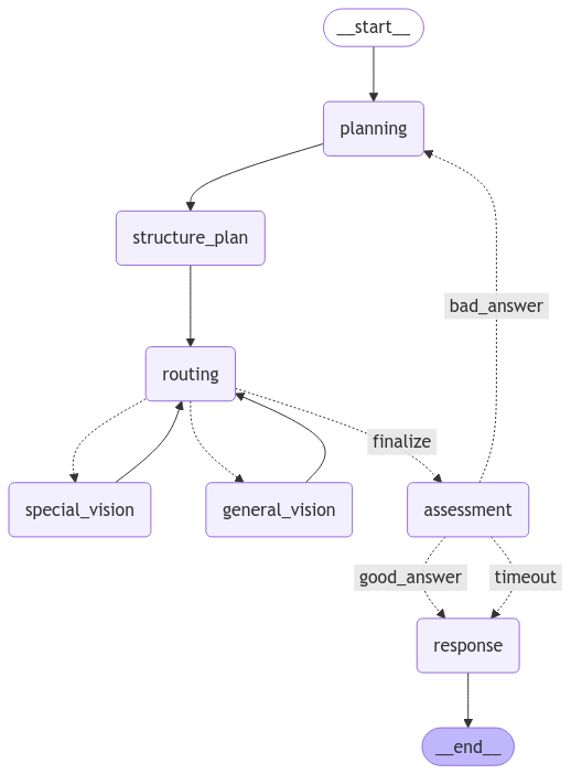
But what exactly is this project? Let’s introduce it with a tour and demo of the system that we’ll build. The StateGraph (take a look at this article for an intro) looks like this, and every query consists of an image and text input.
Visualization of the control flow of the agent that we will build. Image generated by the author.
We proceed through the stages, each of which is associated with a prompt.
Planning. Here the goal is just to formulate a plan in text about how to best answer the questions with the tools available. The prompt contains a list of the tools and their various modes. A more complex system might use RAG at this stage to gather the list of tools most appropriate for the problem and craft a plan
Structure the plan. The aim here is to create a list of plan components that the agent can step through. We take the plan text and force the model to generate a list that is consistently formatted according the Pydantic models here. Its useful to keep both the plan text and the structured plan for evaluation purposes.
Execute the plan. Each element in the structured plan contains a tool name and inputs. We then proceed to call these tools in sequence and gather their results. Our agent has just two available tools: special vision (which calls Florence2) or general vision (which calls Qwen2 or GPT4o) and the routing node is used to keep track of the current plan stage
Assess the result. Once each step of the plan has been executed, a model gets to see the inputs and outputs and make an assessment of whether or not the the question was answered. If not, we go back to the planning step and try to amend the old plan using these new insights. If yes, we proceed to the end. If the model revises the plan too many times, a timeout is triggered that allows the loop to break.
There are many possible improvements and extensions here, for example in the current implementation the agent just spits out the results of all the prior steps, but an LLM could be called here to formulate them into a nice answer if desired.
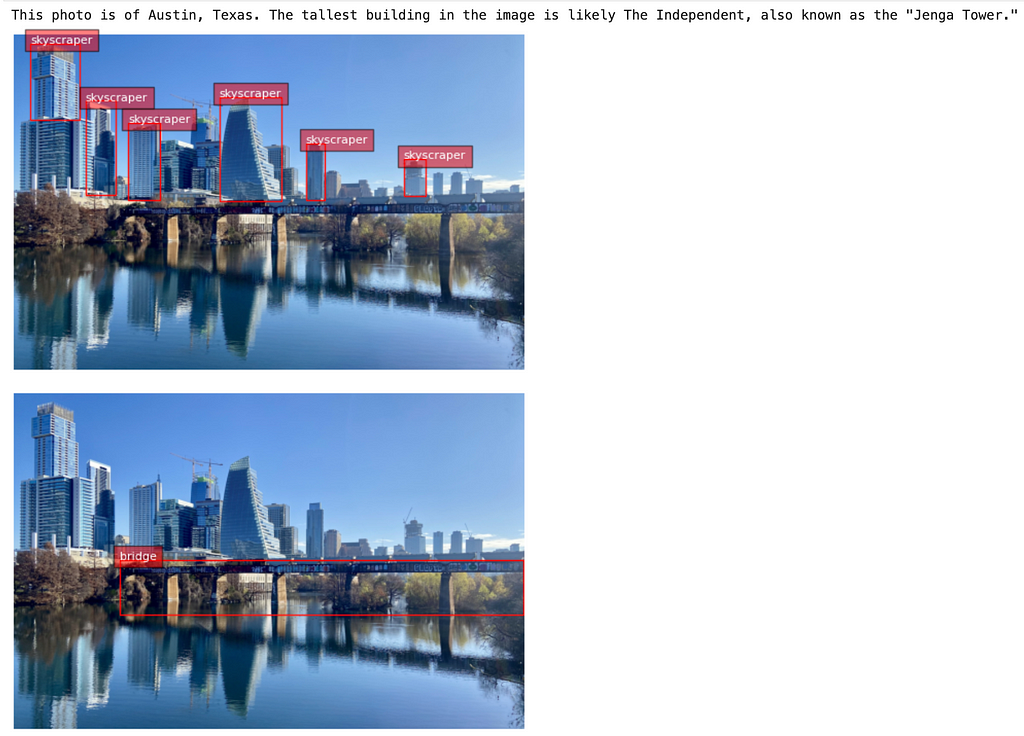
As an example just to see it in action, we give it the following image and input text, which is a fairly complex set of questions
The image used in this example test, photograph taken by the author.
query = """
What city is in this photo? Tell me what the tallest building is, then find all the skyscrapers and bridges
"""
After going through all the steps, this is the result we get.
[
{1: 'This photo is of Austin, Texas. The tallest building in the image is likely The Independent, also known as the "Jenga Tower."'},
{2:
  '{"bboxes": [
    [961.9750366210938, 293.1780090332031, 1253.5550537109375, 783.6420288085938],
    [77.67500305175781, 41.65800094604492, 307.1150207519531, 401.64599609375],
    [335.7950134277344, 310.4700012207031, 474.4150085449219, 753.7739868164062],
    [534.1650390625, 412.6499938964844, 684.7350463867188, 774.2100219726562],
    [1365.885009765625, 510.114013671875, 1454.3150634765625, 774.2100219726562],
    [1824.76513671875, 583.9979858398438, 1927.5350341796875, 758.489990234375]
  ], "labels": ["skyscraper", "skyscraper", "skyscraper", "skyscraper", "skyscraper", "skyscraper"]}'},
{3:
  '{"bboxes": [
    [493.5350341796875, 780.4979858398438, 2386.4150390625, 1035.1619873046875]
  ], "labels": ["bridge"]}'}
}
]
And we can plot these results to confirm the bounding boxes.
The agent’s answer to our multi-part question about this image, where we overlay the bounding box coordinates it provides.
Impressive! One could argue about whether or not it really found all the skyscrapers here but I feel like such a system has the potential to be quite powerful and useful, especially if we were to add the ability to crop the bounding boxes, zoom in and continue the conversation.
In the following sections, let’s dive into the main steps in a bit more detail. My hope is that some of them might be informative for your projects too.
The agent state, nodes and edges
My previous article contains a more detailed discussion of agents and LangGraph, so here I’ll just touch in the agent state for this project. The AgentState is made accessible to all the nodes in the LangGraph graph, and it’s where the information relevant to a query gets stored.
Each node can be told to write to one of more variables in the state, and by default they get overwritten. This is not the behavior we want for the plan output, which is supposed to be a list of results from each step of the plan. To ensure that this list gets appended as the agent goes about its work we use the add reducer, which you can read more about here.
Each of the nodes in the graph above is a method in the class AgentNodes. They take in state, perform some action (typically calling an LLM) and output their updates to the state. As an example, here’s the node used to structure the plan, copied from the code here.
The routing node is also important because it’s visited multiple times over the course of plan execution. In the current code it’s very simple, just updating the current step state value so that other nodes know which part of the plan structure list to look at.
An extension here would be to add another LLM call in the routing node to check if the output of the previous step of the plan warrants any modifications to the next steps or early termination of the question has been answered.
Finally we need to add two conditional edges, which use data stored in the AgentStateto determine which node should be run next. For example, the choose_model edge looks at the name of the current step in the plan_structure object carried in AgentState and then uses a simple if stagement to return the name of corresponding node that should be called at that step.
And it can be vizualized in a notebook using the turorial here.
The orchestration model
The planning, structure and assessment nodes are ideally suited to a text-based LLM that can reason and produce structured outputs. The most straightforward option here is to go with a large, versatile model like GPT4o-mini, which has the benefit of excellent support for JSON output from a Pydantic schema.
With the help of some LangChain functionality, we can make class to call such a model.
from langchain_core.prompts import ChatPromptTemplate from langchain_openai import ChatOpenAI
To set this up, we supply a system prompt and an output model (see here for some examples of these) and then we can just use the call method with an input string to get a response that conforms to the structure of the output model that we specified. With the code set up like this we’d need to make a new instance of StructuredOpenAICaller with every different system prompt and output model we used in the agent. I personally prefer this to keep track of the different models being used, but as the agent becomes more complex it could be modified with another method to directly update the system prompt and output model in the single instance of the class.
Can we do this with local models too? On Apple Silicon, we can use the MLX library and MLX community on Hugging Face to easily experiment with open source models like Llama3.2. LangChain also has support for MLX integration, so we can follow the structure of the class above to set up a local model.
from langchain_core.output_parsers import PydanticOutputParser from langchain_core.prompts import ChatPromptTemplate from langchain_community.llms.mlx_pipeline import MLXPipeline from langchain_community.chat_models.mlx import ChatMLX
class StructuredLlamaCaller: MODEL_PATH = "mlx-community/Llama-3.2-3B-Instruct-4bit"
self.system_prompt = system_prompt # this is the name of the Pydantic model that defines # the structure we want to output self.output_model = output_model self.loaded_model = MLXPipeline.from_model_id( self.MODEL_PATH, pipeline_kwargs={"max_tokens": max_tokens, "temp": temperature, "do_sample": False}, ) self.llm = ChatMLX(llm=self.loaded_model) self.temperature = temperature self.max_tokens = max_tokens self.chain = self._set_up_chain()
def _set_up_chain(self) -> Any: # Set up a parser parser = PydanticOutputParser(pydantic_object=self.output_model)
There are a few interesting points here. For a start, we can just download the weights and config for Llama3.2 as we would any other Hugging Face model, then under the hood they are loaded into MLX using the MLXPipeline tool from LangChain. When the models are first downloaded they are automatically placed in the Hugging Face cache. Sometimes it’s desirable to list the models and their cache locations, for example if you want to copy a model to a new environment. The util scan_cache_dir will help here and can be used to make a useful result with this function.
from huggingface_hub import scan_cache_dir
def fetch_downloaded_model_details():
hf_cache_info = scan_cache_dir()
repo_paths = [] size_on_disk = [] repo_ids = []
for repo in sorted( hf_cache_info.repos, key=lambda repo: repo.repo_path ): repo_paths.append(str(repo.repo_path)) size_on_disk.append(repo.size_on_disk) repo_ids.append(repo.repo_id) repos_df = pd.DataFrame({ "local_path":repo_paths, "size_on_disk":size_on_disk, "model_name":repo_ids })
Llama3.2 does not have a built-in support for structured output like GPT4o-mini, so we need to use the prompt to force it to generate JSON. LangChain’s PydanticOutputParser can help, although it it also possible to implement your own version of this as shown here.
In my experience, the version of Llama that I’m using here, namely Llama-3.2–3B-Instruct-4bit, is not reliable for structured output beyond the simplest schemas. It’s reasonably good at the “plan generation” stage of our agent given a prompt with a few examples, but even with the help of the instructions provided by PydanticOutputParser, it often fails to turn that plan into JSON. Larger and/or less quantized versions of Llama will likely be better, but they would run into RAM issues if run alongside the other models in our agent. Therefore going forwards in the project, the orchestration mdoel is set to be GPT4o-mini.
A model for general vision: Qwen2-VL
To be able to answer questions like “What’s going on in this image?” or “what city is this?”, we need a multimodal LLM. Arguably Florence2 in image captioning mode might be to give good responses to this type of question, but it’s not really designed for conversational output.
The field of multimodal models small enough to run on a laptop is still in its infancy (a recently compiled list can be found here), but the Qwen2-VL series from Alibaba is a promising development. Furthermore, we can make use of MLX-VLM, an extension of MLX specifically designed for tuning and inference of vision models, to set up one of these models within our agent framework.
from mlx_vlm import load, apply_chat_template, generate
class QwenCaller: MODEL_PATH = "mlx-community/Qwen2-VL-2B-Instruct-4bit"
This class will load the smallest version of Qwen2-VL and then call it with an input image and prompt to get a textual response. For more detail about the functionality of this model and others that could be used in the same way, check out this list of examples on the MLX-VLM github page. Qwen2-VL is also apparently capable of generating bounding boxes and object pointing coordinates, so this capability could also be explored and compared with Florence2.
Of course GPT-4o-mini also has vision capabilities and is likely more reliable than smaller local models. Therefore when building these sorts of applications it’s useful to add the ability to call a cloud based alternative, if anything just as a backup in case one of the local models fails. Note that input images must be converted to base64 before they can be sent to the model, but once that’s done we can also use the LangChain framework as shown below.
import base64 from io import BytesIO from PIL import Image from langchain_core.prompts import ChatPromptTemplate from langchain_openai import ChatOpenAI from langchain_core.output_parsers import StrOutputParser
def convert_PIL_to_base64(image: Image, format="jpeg"): buffer = BytesIO() # Save the image to this buffer in the specified format image.save(buffer, format=format) # Get binary data from the buffer image_bytes = buffer.getvalue() # Encode binary data to Base64 base64_encoded = base64.b64encode(image_bytes) # Convert Base64 bytes to string (optional) return base64_encoded.decode("utf-8")
class OpenAIVisionCaller: MODEL_NAME = "gpt-4o-mini"
Florence2 is seen as a specialist model in the context of our agent because while it has many capabilities its inputs must be selected from a list of predefined task prompts. Of course the model could be fine tuned to accept new prompts, but for our purposes the version downloaded directly from Hugging Face works well. The beauty of this model is that it uses a single training process and set of weights, but yet achieves high performance in multiple image tasks that previously would have demanded their own models. The key to this success lies in its large and carefully curated training dataset, FLD-5B. To learn more about the dataset, model and training I recommend this excellent article.
In our context, we use the orchestration model to turn the query into a series of Florence task prompts, which we then call in a sequence. The options available to us include captioning, object detection, phrase grounding, OCR and segmentation. For some of these options (i.e. phrase grounding and region to segmentation) an input phrase is needed, so the orchestration model generates that too. In contrast, tasks like captioning need only the image. There are many use cases for Florence2, which are explored in code here. We restrict ourselves to object detection, phrase grounding, captioning and OCR, though it would be straightforward to add more by updating the prompts associated with plan generation and structuring.
Florence2 appears to be supported by the MLX-VLM package, but at the time of writing I couldn’t find any examples of its use and so opted for an approach that uses Hugging Face transformers as shown below.
from transformers import AutoModelForCausalLM, AutoProcessor import torch
def get_device_type():
if torch.cuda.is_available(): return "cuda" else: if torch.backends.mps.is_available() and torch.backends.mps.is_built(): return "mps" else: return "cpu"
class FlorenceCaller:
MODEL_PATH: str = "microsoft/Florence-2-base-ft" # See https://huggingface.co/microsoft/Florence-2-base-ft for other modes # for Florence2 TASK_DICT: dict[str, str] = { "general object detection": "<OD>", "specific object detection": "<CAPTION_TO_PHRASE_GROUNDING>", "image captioning": "<MORE_DETAILED_CAPTION>", "OCR": "<OCR_WITH_REGION>", }
def __init__(self) -> None: self.device: str = ( get_device_type() ) # Function to determine the device type (e.g., 'cpu' or 'cuda').
# Get the corresponding task code for the given prompt task_code: str = self.translate_task(task_prompt)
# Prevent text_input for tasks that do not require it if task_code in [ "<OD>", "<MORE_DETAILED_CAPTION>", "<OCR_WITH_REGION>", "<DETAILED_CAPTION>", ]: text_input = None
# Construct the prompt based on whether text_input is provided prompt: str = task_code if text_input is None else task_code + text_input
# Preprocess inputs for the model inputs = self.processor(text=prompt, images=image, return_tensors="pt").to( self.device )
# Generate predictions using the model generated_ids = self.model.generate( input_ids=inputs["input_ids"], pixel_values=inputs["pixel_values"], max_new_tokens=1024, early_stopping=False, do_sample=False, num_beams=3, )
# Decode and process generated output generated_text: str = self.processor.batch_decode( generated_ids, skip_special_tokens=False )[0]
On Apple Silicon, the device becomes mps and the latency of these model calls is tolerable. This code should also work on GPU and CPU, though this has not been tested.
Another example and some limitations
Let’s run through another example to see the agent outputs from each step. To call the agent on an input query and image we can use the Agent.invoke method, which follows the same process as described in my previous article to add each node output to a list of results in addition to saving outputs in a LangGraph InMemoryStore object.
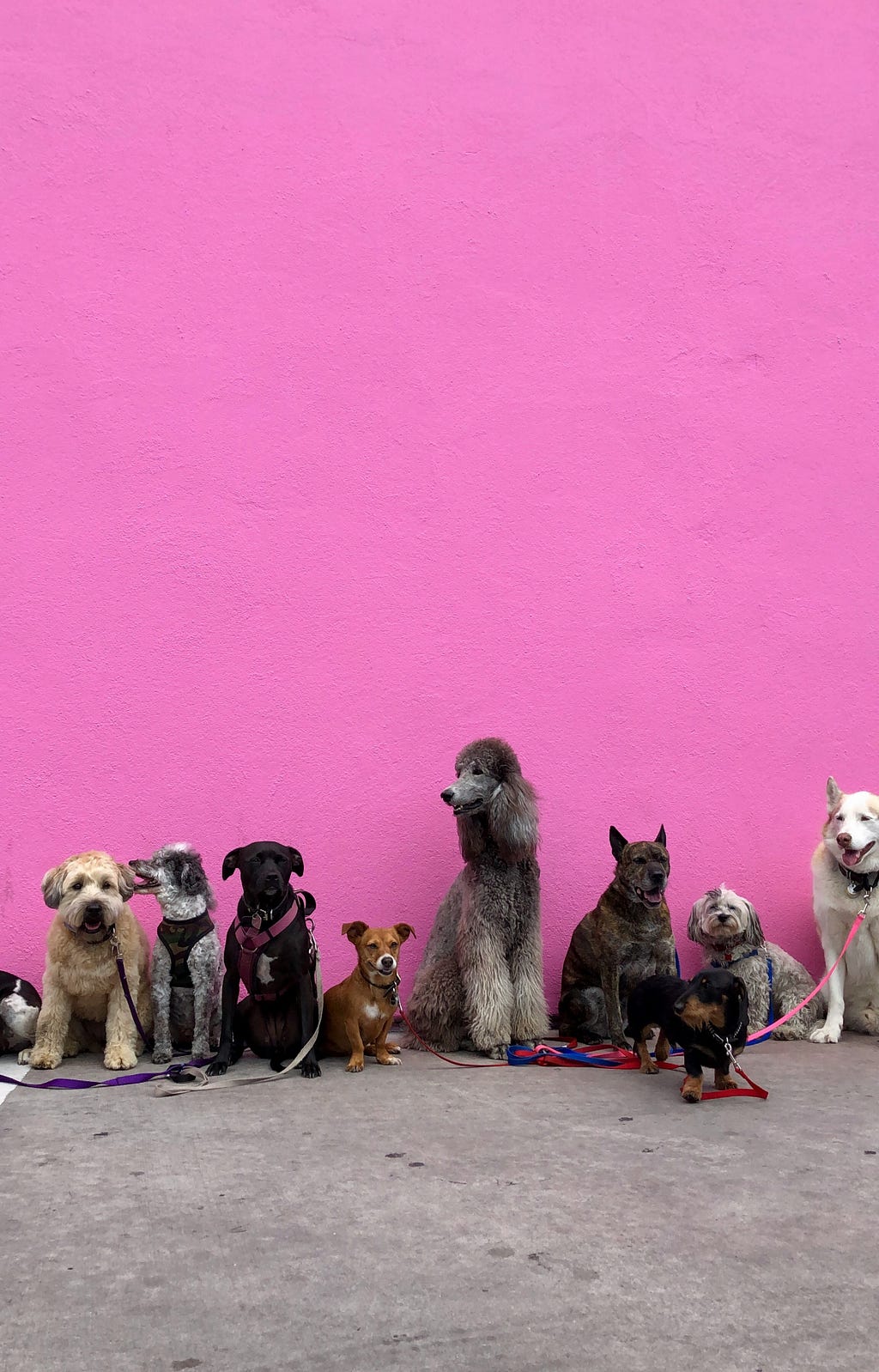
We’ll be using the following image, which presents an interesting challenge if we ask a tricky question like “Are there trees in this image? If so, find them and describe what they are doing”
from image_agent.agent.Agent import Agent
from image_agent.utils import load_secrets

secrets = load_secrets()

# use GPT4 for general vision mode
full_agent_gpt_vision = Agent(
openai_api_key=secrets["OPENAI_API_KEY"],vision_mode="gpt"
)

# use local model for general vision
full_agent_qwen_vision = Agent(
openai_api_key=secrets["OPENAI_API_KEY"],vision_mode="local"
)
In an ideal world the answer is straightforward: There are no trees.
However this turns out to be a difficult question for the agent and it’s interesting to compare the responses when it using GPT-4o-mini vs. Qwen2 as the general vision model.
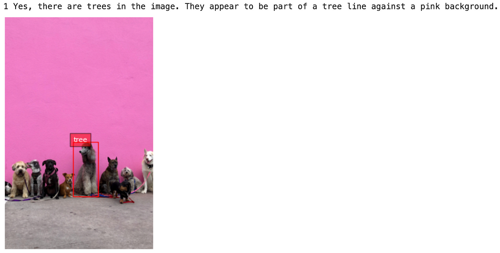
When we call full_agent_qwen_vision with this query, we get a bad result: Both Qwen2 and Florence2 fall for the trick and report that trees are present (interestingly, if we change “trees” to “dogs”, we get the right answer)
Plan:
Call generalist vision with the question 'Are there trees in this image? If so, what are they doing?'. Then call specialist vision in object specific mode with the phrase 'cat'.

Plan_structure:
{
  "1": {"tool_name": "general_vision", "tool_mode": "conversation", "tool_input": "Are there trees in this image? If so, what are they doing?"},
  "2": {"tool_name": "special_vision", "tool_mode": "specific object detection", "tool_input": "tree"}
}

Plan output:
[
  {1: 'Yes, there are trees in the image. They appear to be part of a tree line against a pink background.'}
[
  {2: '{"bboxes": [[235.77601623535156, 427.864501953125, 321.7920227050781, 617.2275390625]], "labels": ["tree"]}'}
]

Assessment:
The result adequately answers the user's question by confirming the presence of trees in the image and providing a description of their appearance and context. The output from both the generalist and specialist vision tools is consistent and informative.
Qwen2 seems subject to blindly following the prompts hint that here might be trees present. Florence2 also fails here, reporting a bounding box when it should not
If asked “Are there trees in this image, If so, find them and describe what they’re doing”, both Qwen2 and Florence2 fall for the trick. Image generated by the author.If asked “Are there dogs in this image? If so, find them and describe what they’re doing”, both the Qwen and GPT-based agents will produce the correct answer. Image generated by the author.
If we call full_agent_gpt_visionwith the same query, GPT4o-mini doesn’t fall for the trick, but the call to Florence2 hasn’t changed so it still fails. We then see the query assessment step in action because the generalist and specialist models have produced conflicting results.
Node : general_vision Task : plan_output [ {1: 'There are no trees in this image. It features a group of dogs sitting in front of a pink wall.'} ]
Node : assessment Task : answer_assessment The result contains conflicting information. The first part states that there are no trees in the image, while the second part provides a bounding box and label indicating that a tree is present. This inconsistency means the user's question is not adequately answered.
The agent then tries several times to restructure the plan, but Florence2 insists on producing a bounding box for “tree”, which the answer assessment nodes always catches as inconsistent. This is a better result than the Qwen2 agent, but points to a broader issue of false positives with Florence2. This could be addressed by having the routing node evaluate the plan after every step and then only call Florence2 if absolutely necessary.
With the basic building blocks in place, this system is ripe for experimentation, iteration and improvement and I may continue to add to the repo over the coming weeks. For now though, this article is long enough!
Thanks for making it to the end and I hope the project here prompts some inspiration for your own projects! The orchestration of multiple specialist models within agent frameworks is a powerful and increasingly accessible approach to putting LLMs to work on complex tasks. Clearly there is still a lot of room for improvI for one look forward to seeing how ideas in this field develop over the coming year.
This is the second article of our GPT series, where we will dive into the development of GPT-2 and GPT-3, with model size increased from 117M to a staggering 175B.
We choose to cover GPT-2 and GPT-3 together not just because they share similar architectures, but also they were developed with a common philosophy aimed at bypassing the finetuning stage in order to make LLMs truly intelligent. Moreover, to achieve that goal, they both explored several key technical elements such as task-agnostic learning, scale hypothesis and in-context learning, etc. Together they demonstrated the power of training large models on large datasets, inspired further research into emergent capabilities, established new evaluation protocols, and sparked discussions on enhancing the safety and ethical aspects of LLMs.
Below are the contents we will cover in this article:
Overview: The paradigm shift towards bypassing finetuning, and the three key elements made this possible: task-agnostic learning, the scaling hypothesis, and in-context learning.
GPT-2: Model architecture, training data, evaluation results, etc.
GPT-3: Core concepts and new findings.
Conclusions.
Overview
The Paradigm Shift Towards Bypassing Finetuning
In our previous article, we revisited the core concepts in GPT-1 as well as what had inspired it. By combining auto-regressive language modeling pre-training with the decoder-only Transformer, GPT-1 had revolutionized the field of NLP and made pre-training plus finetuning a standard paradigm.
But OpenAI didn’t stop there.
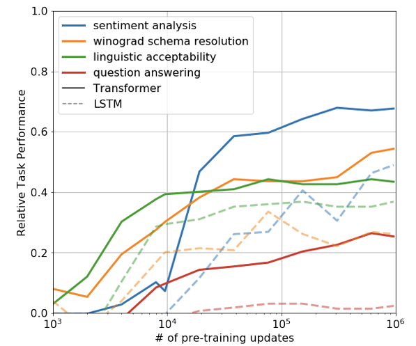
Rather, while they tried to understand why language model pre-training of Transformers is effective, they began to notice the zero-shot behaviors of GPT-1, where as pre-training proceeded, the model was able to steadily improve its performance on tasks that it hadn’t been finetuned on, showing that pre-training could indeed improve its zero-shot capability, as shown in the figure below:
Figure 1. Evolution of zero-shot performance on different tasks as a function of LM pre-training updates. (Image from the GPT-1 paper.)
This motivated the paradigm shift from “pre-training plus finetuning” to “pre-training only”, or in other words, a task-agnostic pre-trained model that can handle different tasks without finetuning.
Both GPT-2 and GPT-3 are designed following this philosophy.
But why, you might ask, isn’t the pre-training plus finetuning magicworking just fine? What are the additional benefits of bypassing the finetuning stage?
Limitations of Finetuning
Finetuning is working fine for some well-defined tasks, but not for all of them, and the problem is that there are numerous tasks in the NLP domain that we have never got a chance to experiment on yet.
For those tasks, the requirement of a finetuning stage means we will need to collect a finetuning dataset of meaningful size for each individual new task, which is clearly not ideal if we want our models to be truly intelligent someday.
Meanwhile, in some works, researchers have observed that there is an increasing risk of exploiting spurious correlations in the finetuning data as the models we are using become larger and larger. This creates a paradox: the model needs to be large enough so that it can absorb as much information as possible during training, but finetuning such a large model on a small, narrowly distributed dataset will make it struggle when generalize to out-of-distribution samples.
Another reason is that, as humans we do not require large supervised datasets to learn most language tasks, and if we want our models to be useful someday, we would like them to have such fluidity and generality as well.
Now perhaps the real question is that, what can we do to achieve that goal and bypass finetuning?
Before diving into the details of GPT-2 and GPT-3, let’s first take a look at the three key elements that have influenced their model design: task-agnostic learning, the scale hypothesis, and in-context learning.
Task-agnostic Learning
Task-agnostic learning, also known as Meta-Learning or Learning to Learn, refers to a new paradigm in machine learning where the model develops a broad set of skills at training time, and then uses these skills at inference time to rapidly adapt to a new task.
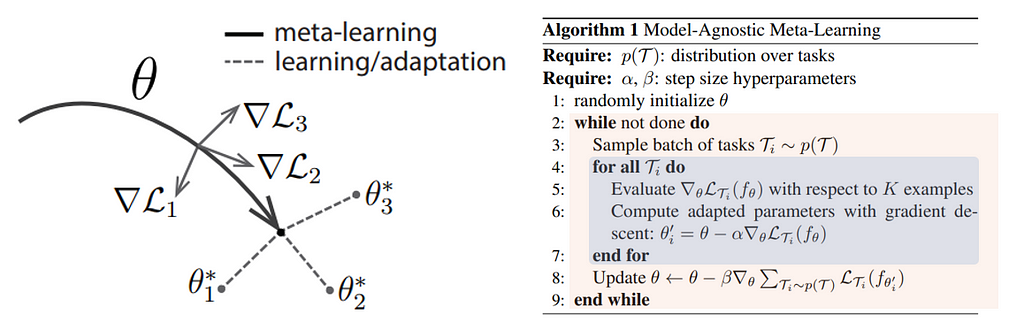
For example, in MAML (Model-Agnostic Meta-Learning), the authors showed that the models could adapt to new tasks with very few examples. More specifically, during each inner loop (highlighted in blue), the model firstly samples a task from a bunch of tasks and performs a few gradient descent steps, resulting in an adapted model. This adapted model will be evaluated on the same task in the outer loop (highlighted in orange), and then the loss will be used to update the model parameters.
Figure 2. Model-Agnostic Meta-Learning. (Image from the MAML paper)
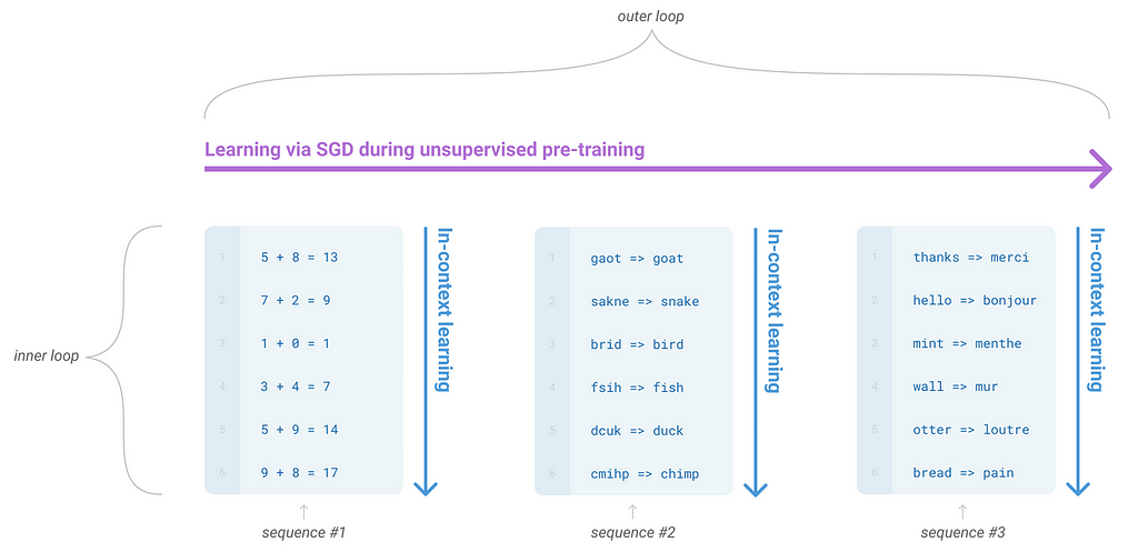
MAML shows that learning could be more general and more flexible, which aligns with the direction of bypassing finetuning on each individual task. In the follow figure the authors of GPT-3 explained how this idea can be extended into learning language models when combined with in-context learning, with the outer loop iterates through different tasks, while the inner loop is described using in-context learning, which will be explained in more detail in later sections.
Figure 3. Language model meta-learning. (Image from GPT-3 paper)
The Scale Hypothesis
As perhaps the most influential idea behind the development of GPT-2 and GPT-3, the scale hypothesis refers to the observations that when training with larger data, large models could somehow develop new capabilities automatically without explicit supervision, or in other words, emergent abilities could occur when scaling up, just as what we saw in the zero-shot abilities of the pre-trained GPT-1.
Both GPT-2 and GPT-3 can be considered as experiments to test this hypothesis, with GPT-2 set to test whether a larger model pre-trained on a larger dataset could be directly used to solve down-stream tasks, and GPT-3 set to test whether in-context learning could bring improvements over GPT-2 when further scaled up.
We will discuss more details on how they implemented this idea in later sections.
In-Context Learning
As we show in Figure 3, under the context of language models, in-context learning refers to the inner loop of the meta-learning process, where the model is given a natural language instruction and a few demonstrations of the task at inference time, and is then expected to complete that task by automatically discovering the patterns in the given demonstrations.
Note that in-context learning happens in the testing phase with no gradient updates performed, which is completely different from traditional finetuning and is more similar to how humans perform new tasks.
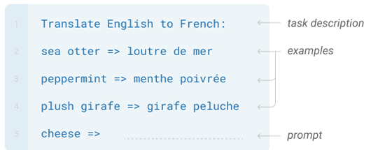
In case you are not familiar with the terminology, demonstrations usually means exemplary input-output pairs associated with a particular task, as we show in the “examples” part in the figure below:
Figure 4. Example of few-shot in-context learning. (Image from GPT-3 paper)
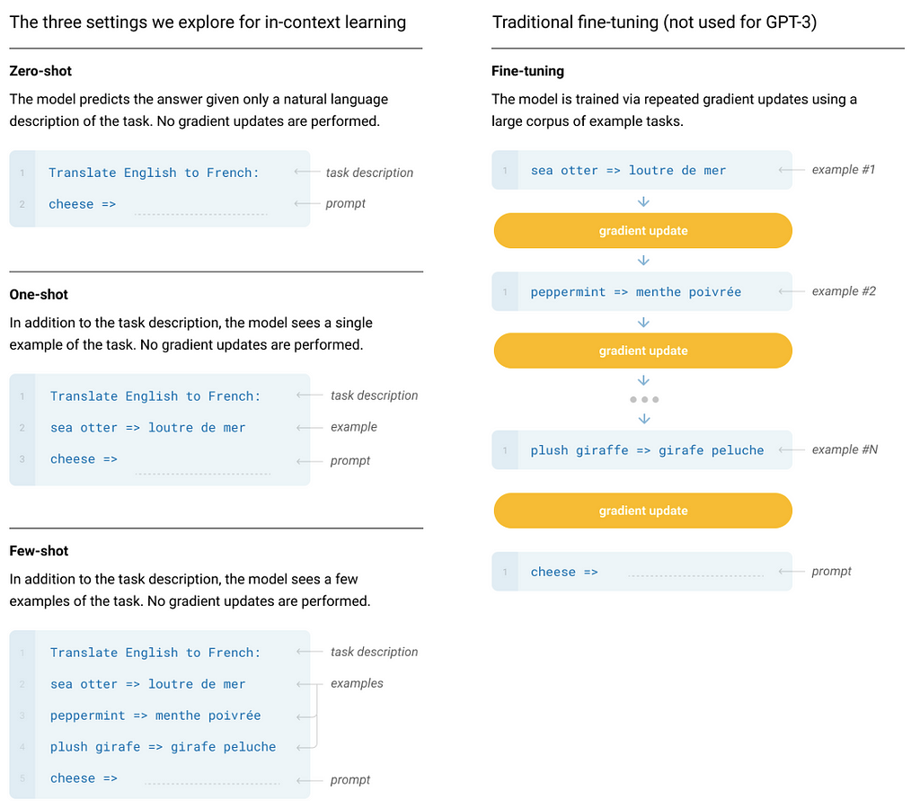
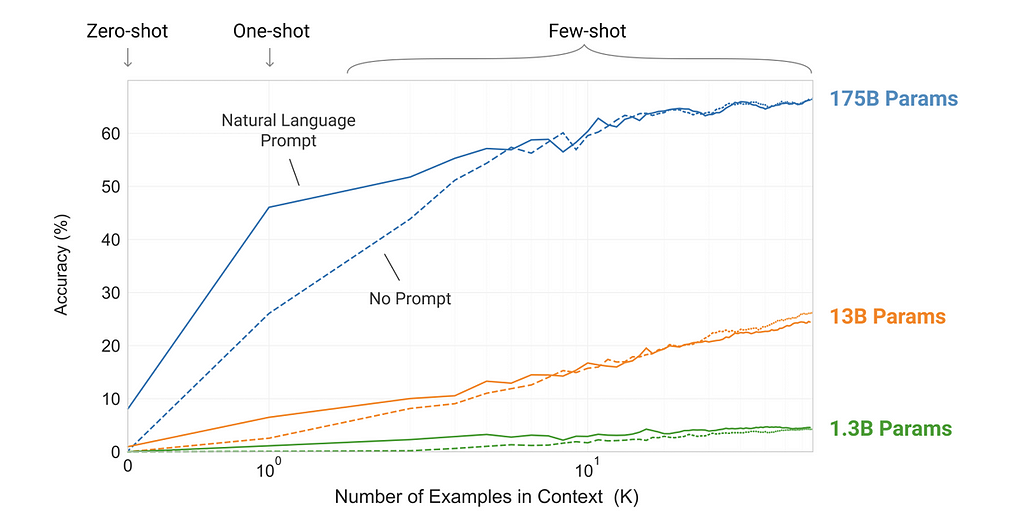
The idea of in-context learning was explored implicitly in GPT-2 and then more formally in GPT-3, where the authors defined three different settings: zero-shot, one-shot, and few-shot, depending on how many demonstrations are given to the model.
Figure 5. zero-shot, one-shot and few-shot in-context learning, contrasted with traditional finetuning. (Image from GPT-3 paper)
In short, task-agnostic learning highlights the potential of bypassing finetuning, while the scale hypothesis and in-context learning suggest a practical path to achieve that.
In the following sections, we will walk through more details for GPT-2 and GPT-3, respectively.
GPT-2
Model Architecture
The GPT-2 model architecture is largely designed following GPT-1, with a few modifications:
Moving LayerNorm to the input of each sub-block and adding an additional LayerNorm after the final self-attention block to make the training more stable.
Scaling the weights of the residual layers by a factor of 1/sqrt(N), where N is the number of residual layers.
Expanding the vocabulary to 50257, and also using a modified BPE vocabulary.
Increasing context size from 512 to 1024 tokens and using a larger batch size of 512.
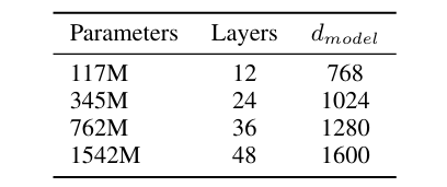
In the GPT-2 paper, the authors trained four models with approximately log-uniformly spaced sizes, with number of parameter ranging from 117M to 1.5B:
Table 1. Architecture hyperparameters for 4 GPT-2 models. (Image from GPT-2 paper)
Training Data
As we scale up the model we also need to use a larger dataset for training, and that is why in GPT-2 the authors created a new dataset called WebText, which contains about 45M links and is much larger than that used in pre-training GPT-1. They also mentioned lots of techniques to cleanup the data to improve its quality.
Evaluation Results
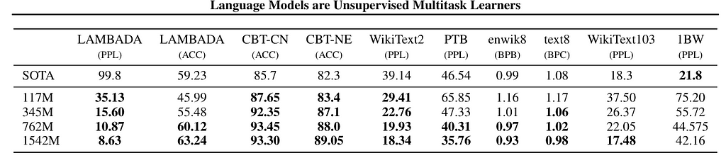
Overall, GPT-2 achieved good results on many tasks, especially for language modeling related ones. However, for tasks like reading comprehension, translation and QA, it still performed worse than the respective SOTA models, which partly motivates the development of GPT-3.
Table 2. GPT-2 zero-shot performance. (Image from GPT-2 paper)
GPT-3
Model Architecture
GPT-3 adopted a very similar model architecture to that of GPT-2, and the only difference is that GPT-3 used an alternating dense and locally banded sparse attention patterns in Transformer.
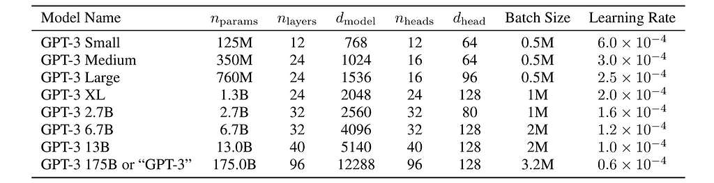
GPT-3 trained 8 models with different sizes, with number of parameters ranging from 125M to 175B:
Table 3. Architecture hyperparameters for 8 GPT-3 models. (Image from GPT-3 paper)
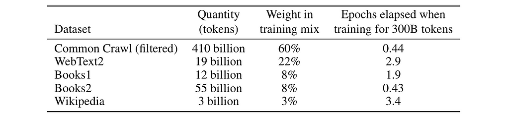
Training Data
GPT-3 model was trained on even larger datasets, as listed in the table below, and again the authors did some cleanup work to improve data quality. Meanwhile, training datasets were not sampled in proportion to their size, but rather according to their quality, with high-quality dataset sampled more frequently during training.
Table 4. Datasets used in GPT-3 training. (Image from GPT-3 paper)
Evaluation Results
By combining larger model with in-context learning, GPT-3 achieved strong performance on many NLP datasets including translation, question-answering, cloze tasks, as well as tasks require on-the-fly reasoning or domain adaptation. The authors presented very detailed evaluation results in the original paper.
A few findings that we want to highlight in this article:
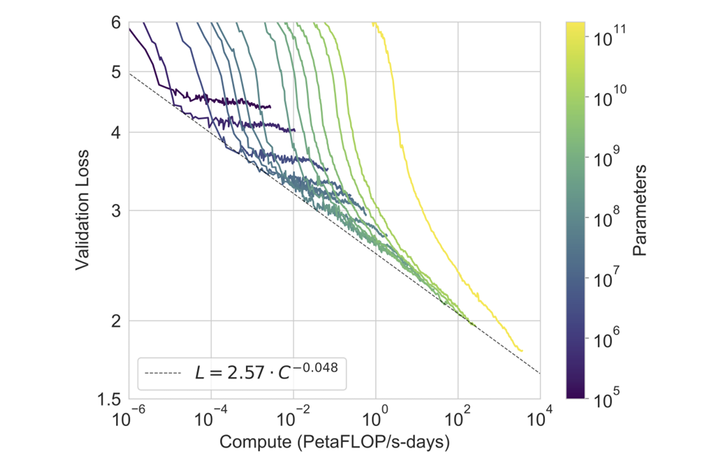
Firstly, during training of GPT-3 they observed a smooth scaling trend of performance with compute, as shown in the figure below, where the validation loss decreases linearly as compute increasing exponentially.
Figure 6. Smooth scaling of performance with compute. (Image from GPT-3 paper)
Secondly, when comparing the three in-context learning settings (zero-shot, one-shot and few-shot), they observed that larger models appeared more efficient in all the three settings:
Figure 7. Larger models are more efficient in in-context learning. (Image from GPT-3 paper)
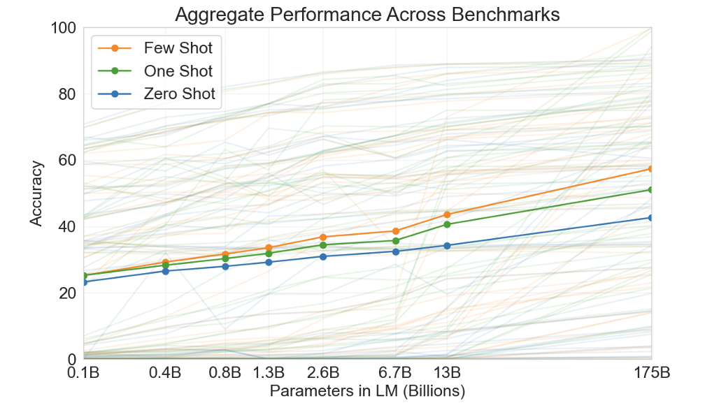
Following that, they plotted the aggregate performance for all the three settings, which further demonstrated that larger models are more effective, and few-shot performance increased more rapidly than the other two settings.
Figure 8. Aggregate performance for all 42 accuracy-denominated benchmarks. (Image from GPT-3 paper)
Conclusions
The development of GPT-2 and GPT-3 bridges the gap between the original GPT-1 with more advanced versions like InstructGPT, reflecting the ongoing refinement of OpenAI’s methodology in training useful LLMs.
Their success also paves the way for new research directions in both NLP and the broader ML community, with many subsequent works focusing on understanding emergent capabilities, developing new training paradigms, exploring more effective data cleaning strategies, and proposing effective evaluation protocols for aspects like safety, fairness, and ethical considerations, etc.
In the next article, we will continue our exploration and walk you through the key elements of GPT-3.5 and InstructGPT.
The Education and Training Quality Authority (BQA) plays a critical role in improving the quality of education and training services in the Kingdom Bahrain. BQA reviews the performance of all education and training institutions, including schools, universities, and vocational institutes, thereby promoting the professional advancement of the nation’s human capital. In this post, we explore how BQA used the power of Amazon Bedrock, Amazon SageMaker JumpStart, and other AWS services to streamline the overall reporting workflow.
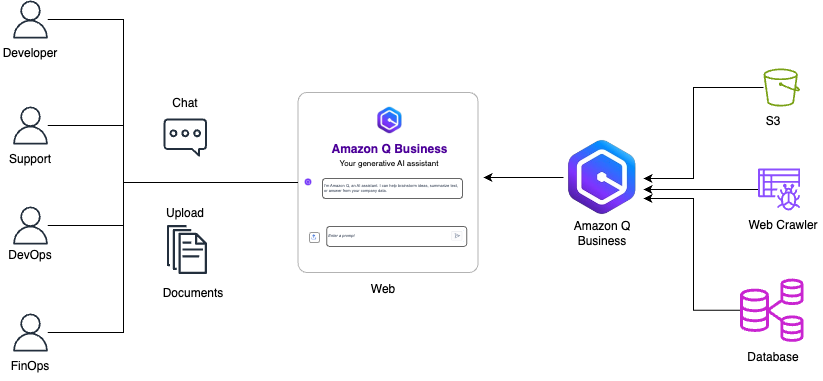
This post shows how MuleSoft introduced a generative AI-powered assistant using Amazon Q Business to enhance their internal Cloud Central dashboard. This individualized portal shows assets owned, costs and usage, and well-architected recommendations to over 100 engineers.
Eindhoven-based startup Photon IP has raised €4.75mn in seed funding as it looks to scale up its unique method for creating energy-efficient photonic chips. AI systems, data centres, fibre-optic networks, and even some sensors rely on photonic chips to send and receive information using light. These chips are a big deal because they’re faster and use less energy than typical semiconductors, which transfer data through electricity. But to make these high-performance, light-speed chips you need special compounds called III-V materials, such as indium phosphide. “These materials are relatively scarce and expensive though, so the industry has been looking at ways of…
We use cookies on our website to give you the most relevant experience by remembering your preferences and repeat visits. By clicking “Accept”, you consent to the use of ALL the cookies.
This website uses cookies to improve your experience while you navigate through the website. Out of these, the cookies that are categorized as necessary are stored on your browser as they are essential for the working of basic functionalities of the website. We also use third-party cookies that help us analyze and understand how you use this website. These cookies will be stored in your browser only with your consent. You also have the option to opt-out of these cookies. But opting out of some of these cookies may affect your browsing experience.
Necessary cookies are absolutely essential for the website to function properly. These cookies ensure basic functionalities and security features of the website, anonymously.
Cookie
Duration
Description
cookielawinfo-checkbox-analytics
11 months
This cookie is set by GDPR Cookie Consent plugin. The cookie is used to store the user consent for the cookies in the category "Analytics".
cookielawinfo-checkbox-functional
11 months
The cookie is set by GDPR cookie consent to record the user consent for the cookies in the category "Functional".
cookielawinfo-checkbox-necessary
11 months
This cookie is set by GDPR Cookie Consent plugin. The cookies is used to store the user consent for the cookies in the category "Necessary".
cookielawinfo-checkbox-others
11 months
This cookie is set by GDPR Cookie Consent plugin. The cookie is used to store the user consent for the cookies in the category "Other.
cookielawinfo-checkbox-performance
11 months
This cookie is set by GDPR Cookie Consent plugin. The cookie is used to store the user consent for the cookies in the category "Performance".
viewed_cookie_policy
11 months
The cookie is set by the GDPR Cookie Consent plugin and is used to store whether or not user has consented to the use of cookies. It does not store any personal data.
Functional cookies help to perform certain functionalities like sharing the content of the website on social media platforms, collect feedbacks, and other third-party features.
Performance cookies are used to understand and analyze the key performance indexes of the website which helps in delivering a better user experience for the visitors.
Analytical cookies are used to understand how visitors interact with the website. These cookies help provide information on metrics the number of visitors, bounce rate, traffic source, etc.
Advertisement cookies are used to provide visitors with relevant ads and marketing campaigns. These cookies track visitors across websites and collect information to provide customized ads.