Bitget Wallet will prioritize its native BGB token for multi-chain gas payments via its innovative GetGas feature starting January 2025, according to a Dec. 27 statement shared with CryptoSlate. This initiative is set to streamline operations across multiple blockchains, including Ethereum, Solana, BNB Chain, Polygon, Base, Arbitrum, Optimism, TON, and Tron. According to the firm, […]
The US Department of the Treasury and the Internal Revenue Service (IRS) have released the final version of its broker rules to digital assets services providers, which includes provisions on requiring DeFi protocols to conduct Know-Your-Customer (KYC) procedures. Industry experts have already criticized the new provision for being unlawful and out of the Treasury’s regulatory […]
Bitcoin’s Spot ETF segment is heating up, with Bitwise’s latest application the most recent example
Post-festive season flows look to be adopting a positive shift after recent ETF outflows
At press time, 69.2% of top traders on Binance held long positions in THETA
THETA’s Relative Strength Index (RSI) stood at 43, indicating a potential for upside momentum
Introduction to the Finite Normal Mixtures in Regression with R
How to make linear regression flexible enough for non-linear data
The linear regression is usually considered not flexible enough to tackle the nonlinear data. From theoretical viewpoint it is not capable to dealing with them. However, we can make it work for us with any dataset by using finite normal mixtures in a regression model. This way it becomes a very powerful machine learning tool which can be applied to virtually any dataset, even highly non-normal with non-linear dependencies across the variables.
What makes this approach particularly interesting comes with interpretability. Despite an extremely high level of flexibility all the detected relations can be directly interpreted. The model is as general as neural network, still it does not become a black-box. You can read the relations and understand the impact of individual variables.
In this post, we demonstrate how to simulate a finite mixture model for regression using Markov Chain Monte Carlo (MCMC) sampling. We will generate data with multiple components (groups) and fit a mixture model to recover these components using Bayesian inference. This process involves regression models and mixture models, combining them with MCMC techniques for parameter estimation.
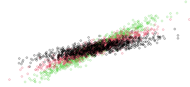
Data simulated as a mixtures of three linear regressions
Loading Required Libraries
We begin by loading the necessary libraries to work with regression models, MCMC, and multivariate distributions
# Loading the required libraries for various functions
library("pscl")         # For pscl specific functions, like regression models
library("MCMCpack")     # For MCMC sampling functions, including posterior distributions
library(mvtnorm)        # For multivariate normal distribution functio
pscl: Used for various statistical functions like regression models.
MCMCpack: Contains functions for Bayesian inference, particularly MCMC sampling.
mvtnorm: Provides tools for working with multivariate normal distributions.
Data Generation
We simulate a dataset where each observation belongs to one of several groups (components of the mixture model), and the response variable is generated using a regression model with random coefficients.
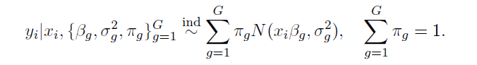
We consider a general setup for a regression model using G Normal mixture components.
## Generate the observations
# Set the length of the time series (number of observations per group)
N <- 1000
# Set the number of simulations (iterations of the MCMC process)
nSim <- 200
# Set the number of components in the mixture model (G is the number of groups)
G <- 3
N: The number of observations per group.
nSim: The number of MCMC iterations.
G: The number of components (groups) in our mixture model.
Simulating Data
Each group is modeled using a univariate regression model, where the explanatory variables (X) and the response variable (y) are simulated from normal distributions. The betas represent the regression coefficients for each group, and sigmas represent the variance for each group.
# Set the values for the regression coefficients (betas) for each group
betas <- 1:sum(dimG) * 2.5  # Generating sequential betas with a multiplier of 2.5
# Define the variance (sigma) for each component (group) in the mixture
sigmas <- rep(1, G) / 1  # Set variance to 1 for each component, with a fixed divisor of 1
betas: These are the regression coefficients. Each group’s coefficient is sequentially assigned.
sigmas: Represents the variance for each group in the mixture model.
In this model we allow each mixture component to possess its own variance paraameter and set of regression parameters.
Group Assignment and Mixing
We then simulate the group assignment of each observation using a random assignment and mix the data for all components.
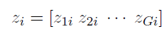
We augment the model with a set of component label vectors for
where
and thus z_gi=1 implies that the i-th individual is drawn from the g-th component of the mixture.
This random assignment forms the z_original vector, representing the true group each observation belongs to.
# Initialize the original group assignments (z_original)
z_original <- matrix(NA, N * G, 1)
# Repeat each group label N times (assign labels to each observation per group)
z_original <- rep(1:G, rep(N, G))
# Resample the data rows by random order
sampled_order <- sample(nrow(data))
# Apply the resampled order to the data
data <- data[sampled_order,]
Bayesian Inference: Priors and Initialization
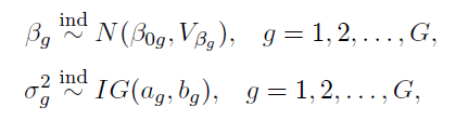
We set prior distributions for the regression coefficients and variances. These priors will guide our Bayesian estimation.
## Define Priors for Bayesian estimation# Define the prior mean (muBeta) for the regression coefficients
muBeta <- matrix(0, G, 1)# Define the prior variance (VBeta) for the regression coefficients
VBeta <- 100 * diag(G)  # Large variance (100) as a prior for the beta coefficients# Prior for the sigma parameters (variance of each component)
ag <- 3  # Shape parameter
bg <- 1/2  # Rate parameter for the prior on sigma
shSigma <- ag
raSigma <- bg^(-1)
muBeta: The prior mean for the regression coefficients. We set it to 0 for all components.
VBeta: The prior variance, which is large (100) to allow flexibility in the coefficients.
shSigma and raSigma: Shape and rate parameters for the prior on the variance (sigma) of each group.
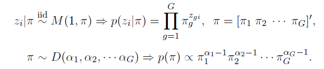
For the component indicators and component probabilities we consider following prior assignment
The multinomial prior M is the multivariate generalizations of the binomial, and the Dirichlet prior D is a multivariate generalization of the beta distribution.
MCMC Initialization
In this section, we initialize the MCMC process by setting up matrices to store the samples of the regression coefficients, variances, and mixing proportions.
## Initialize MCMC sampling# Initialize matrix to store the samples for beta
mBeta <- matrix(NA, nSim, G)# Assign the first value of beta using a random normal distribution
for (g in 1:G) {
  mBeta[1, g] <- rnorm(1, muBeta[g, 1], VBeta[g, g])
}# Initialize the sigma^2 values (variance for each component)
mSigma2 <- matrix(NA, nSim, G)
mSigma2[1, ] <- rigamma(1, shSigma, raSigma)# Initialize the mixing proportions (pi), using a Dirichlet distribution
mPi <- matrix(NA, nSim, G)
alphaPrior <- rep(N/G, G)  # Prior for the mixing proportions, uniform across groups
mPi[1, ] <- rdirichlet(1, alphaPrior)
mBeta: Matrix to store samples of the regression coefficients.
mSigma2: Matrix to store the variances (sigma squared) for each component.
mPi: Matrix to store the mixing proportions, initialized using a Dirichlet distribution.
MCMC Sampling: Posterior Updates
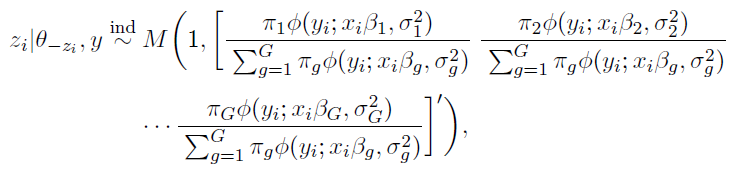
If we condition on the values of the component indicator variables z, the conditional likelihood can be expressed as
In the MCMC sampling loop, we update the group assignments (z), regression coefficients (beta), and variances (sigma) based on the posterior distributions. The likelihood of each group assignment is calculated, and the group with the highest posterior probability is selected.
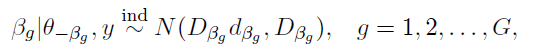
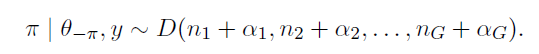
The following complete posterior conditionals can be obtained:
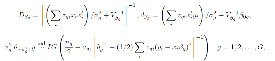
where
denotes all the parameters in our posterior other than x.
and where n_g denotes the number of observations in the g-th component of the mixture.
and
Algorithm below draws from the series of posterior distributions above in a sequential order.
## Start the MCMC iterations for posterior sampling# Loop over the number of simulations
for (i in 2:nSim) {
  print(i)  # Print the current iteration number

  # For each observation, update the group assignment (z)
  for (t in 1:(N*G)) {
    fig <- NULL
    for (g in 1:G) {
      # Calculate the likelihood of each group and the corresponding posterior probability
      fig[g] <- dnorm(y[t, 1], X[t, ] %*% mBeta[i-1, g], sqrt(mSigma2[i-1, g])) * mPi[i-1, g]
    }
    # Avoid zero likelihood and adjust it
    if (all(fig) == 0) {
      fig <- fig + 1/G
    }

    # Sample a new group assignment based on the posterior probabilities
    z[i, t] <- which(rmultinom(1, 1, fig/sum(fig)) == 1)
  }

  # Update the regression coefficients for each group
  for (g in 1:G) {
    # Compute the posterior mean and variance for beta (using the data for group g)
    DBeta <- solve(t(X[z[i, ] == g, ]) %*% X[z[i, ] == g, ] / mSigma2[i-1, g] + solve(VBeta[g, g]))
    dBeta <- t(X[z[i, ] == g, ]) %*% y[z[i, ] == g, 1] / mSigma2[i-1, g] + solve(VBeta[g, g]) %*% muBeta[g, 1]

    # Sample a new value for beta from the multivariate normal distribution
    mBeta[i, g] <- rmvnorm(1, DBeta %*% dBeta, DBeta)

    # Update the number of observations in group g
    ng[i, g] <- sum(z[i, ] == g)

    # Update the variance (sigma^2) for each group
    mSigma2[i, g] <- rigamma(1, ng[i, g]/2 + shSigma, raSigma + 1/2 * sum((y[z[i, ] == g, 1] - (X[z[i, ] == g, ] * mBeta[i, g]))^2))
  }

  # Reorder the group labels to maintain consistency
  reorderWay <- order(mBeta[i, ])
  mBeta[i, ] <- mBeta[i, reorderWay]
  ng[i, ] <- ng[i, reorderWay]
  mSigma2[i, ] <- mSigma2[i, reorderWay]

  # Update the mixing proportions (pi) based on the number of observations in each group
  mPi[i, ] <- rdirichlet(1, alphaPrior + ng[i, ])
}
This block of code performs the key steps in MCMC:
Group Assignment Update: For each observation, we calculate the likelihood of the data belonging to each group and update the group assignment accordingly.
Regression Coefficient Update: The regression coefficients for each group are updated using the posterior mean and variance, which are calculated based on the observed data.
Variance Update: The variance of the response variable for each group is updated using the inverse gamma distribution.
Visualizing the Results
Finally, we visualize the results of the MCMC sampling. We plot the posterior distributions for each regression coefficient, compare them to the true values, and plot the most likely group assignments.
# Plot the posterior distributions for each beta coefficient
par(mfrow=c(G,1))
for (g in 1:G) {
  plot(density(mBeta[5:nSim, g]), main = 'True parameter (vertical) and the distribution of the samples')  # Plot the density for the beta estimates
  abline(v = betas[g])  # Add a vertical line at the true value of beta for comparison
}
This plot shows how the MCMC samples (posterior distribution) for the regression coefficients converge to the true values (betas).
Conclusion
Through this process, we demonstrated how finite normal mixtures can be used in a regression context, combined with MCMC for parameter estimation. By simulating data with known groupings and recovering the parameters through Bayesian inference, we can assess how well our model captures the underlying structure of the data.
Unless otherwise noted, all images are by the author.
The lowest price on Apple’s iPad mini 7 can be found at B&H and Amazon, with both retailers running a limited-time deal on the 256GB model.
Save $70 on Apple’s iPad mini 7 with 256GB capacity.
The 256GB iPad mini 7 in Space Gray can be snapped up for $529 at B&H and Amazon today, with both retailers knocking $70 off Apple’s MSRP on the Wi-Fi model.
Charles really loves his mostly-older Apple gear, but 2025 is going to be a year of change. Here’s how he gets work done at AppleInsider.
The AppleInsider weekend news hub and Zoom/podcasting studio.
I only develop and write stories for AppleInsider on the weekends, hence my Weekend Editor title. As a result, I have a pretty modest setup and workflow compared to most of the full-timers.
Versatility for travel is one of my key requirements, since I am on the road at various times of the year. Even when I’m at home, I’m often in a cafe or occasionally doing local radio as a “computer guru,” or on Zoom teaching online tech classes.
We use cookies on our website to give you the most relevant experience by remembering your preferences and repeat visits. By clicking “Accept”, you consent to the use of ALL the cookies.
This website uses cookies to improve your experience while you navigate through the website. Out of these, the cookies that are categorized as necessary are stored on your browser as they are essential for the working of basic functionalities of the website. We also use third-party cookies that help us analyze and understand how you use this website. These cookies will be stored in your browser only with your consent. You also have the option to opt-out of these cookies. But opting out of some of these cookies may affect your browsing experience.
Necessary cookies are absolutely essential for the website to function properly. These cookies ensure basic functionalities and security features of the website, anonymously.
Cookie
Duration
Description
cookielawinfo-checkbox-analytics
11 months
This cookie is set by GDPR Cookie Consent plugin. The cookie is used to store the user consent for the cookies in the category "Analytics".
cookielawinfo-checkbox-functional
11 months
The cookie is set by GDPR cookie consent to record the user consent for the cookies in the category "Functional".
cookielawinfo-checkbox-necessary
11 months
This cookie is set by GDPR Cookie Consent plugin. The cookies is used to store the user consent for the cookies in the category "Necessary".
cookielawinfo-checkbox-others
11 months
This cookie is set by GDPR Cookie Consent plugin. The cookie is used to store the user consent for the cookies in the category "Other.
cookielawinfo-checkbox-performance
11 months
This cookie is set by GDPR Cookie Consent plugin. The cookie is used to store the user consent for the cookies in the category "Performance".
viewed_cookie_policy
11 months
The cookie is set by the GDPR Cookie Consent plugin and is used to store whether or not user has consented to the use of cookies. It does not store any personal data.
Functional cookies help to perform certain functionalities like sharing the content of the website on social media platforms, collect feedbacks, and other third-party features.
Performance cookies are used to understand and analyze the key performance indexes of the website which helps in delivering a better user experience for the visitors.
Analytical cookies are used to understand how visitors interact with the website. These cookies help provide information on metrics the number of visitors, bounce rate, traffic source, etc.
Advertisement cookies are used to provide visitors with relevant ads and marketing campaigns. These cookies track visitors across websites and collect information to provide customized ads.