A fresh class action suit has been lodged against Binance, accusing the company and its founder, Changpeng Zhao, of failing to prevent money laundering on the platform.
Fanton Fantasy Football is thrilled to announce the successful completion of a significant seed funding round, securing $1M. This innovative blockchain-based fantasy sports platform is seamlessly integrated into Telegram, offering an exciting and immersive experience for users. Notable blockchain and venture capital figures joined forces in this significant investment round. Participants included Animoca Brands, Delphi […]
You have probably seen or interacted with a graph whether you realize it or not. Our world is composed of relationships. Who we know, how we interact, how we transact — graphs structure information in a way that makes these inherent relationships explicit.
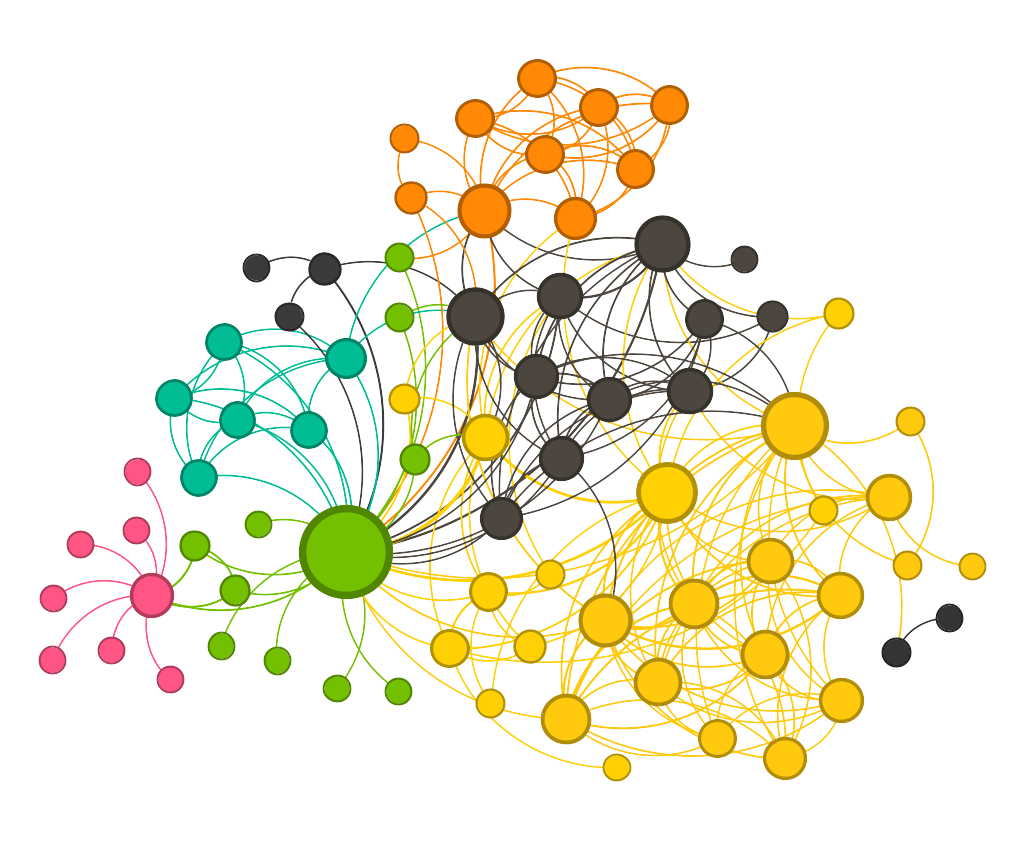
Analytically speaking, knowledge graphs provide the most intuitive means to synthesize and represent connections within and across datasets for analysis. A knowledge graph is a technical artifact “that presents data visually as entities and the relationships between them.” It gives an analyst a digital model of a problem. And it looks something like this…
Image by Author
This article discusses what makes a great graph and answers some common questions pertaining to their technical implementation.
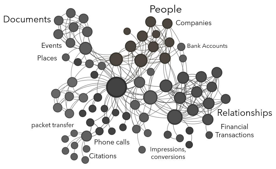
Graphs can represent almost anything where there is interaction or exchange. Entities (or nodes) can be people, companies, documents, geographic locations, bank accounts, crypto wallets, physical assets, etc. Edges (or links) can represent conversations, phone calls, e-mails, academic citations, network packet transfer, ad impressions and conversions, financial transactions, personal relationships, etc.
Image by Author
So what makes a great graph?
The purpose of the graph is clear.
The domain of graph-based solutions includes an analytical environment (often powered by a graph database), graph analytic techniques, and graph visualization techniques. Graphs, like most analytic tools, require specific use cases. Graphs can be used to visualize connections within and across datasets, to discover latent connections, to simulate the dissemination of information or model contagion, to model network traffic or social behavior, to identify most influential actors in a social network, and many other use cases. Who is using the graph? What are these users trying to accomplish analytically and/or visually? Are they exploring an organization’s data? Are they answering specific questions? Are they analyzing, modeling, simulating, predicting? Understanding the use cases the graph-based solution needs to address is the first step to establishing the purpose of the graph and identifying the graph’s domain.
The graph is domain-specific.
Probably the biggest mistake in implementing graph-based solutions is the attempt to create the master graph. One Graph to Rule Them All. In other words, all enterprise data in one graph. Graph is not a Master Data Management (MDM) solution nor is it a replacement for a data warehouse, even if the organization has a scalable graph database in place. The most successful graphs represent a given domain of analytic inquiry. For example, a financial intelligence graph may contain companies, beneficial ownership structures, financial transactions, financial institutions, and high net worth individuals. A pattern-of-life locational graph may contain high-volume signals data such as IP addresses and mobile phone data, alongside physical locations, technical assets, and individuals. Once a graph’s purpose and domain are clear, architects can move on to the data available and/or required to construct the graph.
The graph has a clear schema.
A graph that lives in a graph database will have a schema that dictates its structure. In other words, the schema will specify the types of entities that exist in the graph and the relationships that are permitted between them. One benefit of a graph database over other database types is that the schema is flexible and can be updated as new data, entities, and relationship types are added to the graph over time. Graph data engineers make many decisions when designing a graph database to represent the ontology — the conceptual structure of a dataset — in a schema that makes sense for the graph being created. If the data are well understood in the organization, frequently the graph architecting process can begin with schema creation, but if the nature of the graph and inclusive datasets is more exploratory, ontology design may be required first.
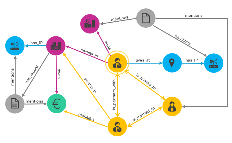
Consider the sample schema in the image below. There are five entity types: people (yellow), physical and virtual locations (blue), documents (gray), companies (pink), and financial accounts (green). Between entities, several relationship types are permitted, e.g., “is_related_to”, “mentions”, and “invests_in”. This is a directed graph meaning that the directionality of the relationship has meaning, i.e., two people are_married_to each other (bidirectional link) and a person lives_at a place (directed link).
Image by Author
There is a clear mechanism for connecting datasets.
Connections between entities across datasets may not always be explicit in the data. Simply importing two datasets into a graph environment could result in many nodes with no connections between them.
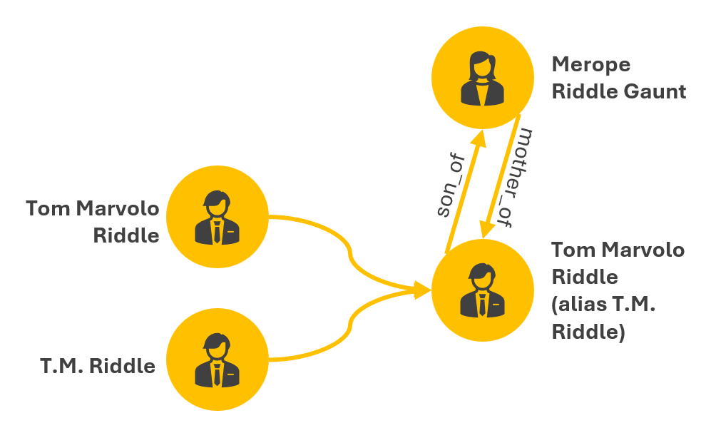
Consider a medical dataset that has a Tom Marvolo Riddle entry and a voter registration dataset that has a T.M. Riddle entry and a Merope Riddle Gaunt entry. In the medical dataset, Merope Gaunt is listed as Tom Riddle’s mother. In the voter registration dataset, there are no family members described. How do the Tom Marvolo Riddle and T.M. Riddle entries get deduplicated when merging the datasets in the graph?, i.e., there should not be two separate nodes in the graph for Tom Riddle and T.M. Riddle as they are the same person. How do Tom Riddle and Merope Gaunt get connected, and how is their connection specified as in the image below?, e.g., connected, related, mother/son? Is the relationship weighted?
These questions require not only a data engineering team to specify the graph schema and implement the graph’s design, but also some sort of entity resolution process, which I have written about previously.
Image by Author
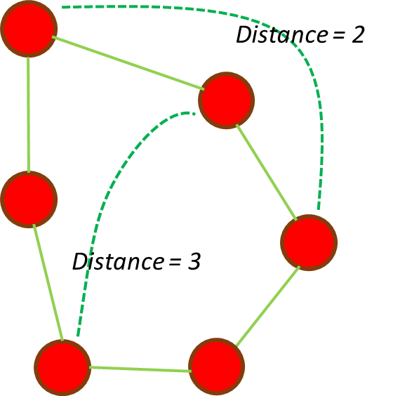
The graph is architected to scale.
Graph data are pre-joined in graph data storage, meaning that one-hop queries run faster than in traditional databases, e.g., query Tom Riddle and see all of his immediate connections. Analytical operations on graphs, however, are quite slow, e.g., ‘show me the shortest path between Tom Riddle and Minerva McGonagall’, or ‘which character has the highest eigenvector centrality in Harry Potter and the Half Blood Prince’? As a general rule, latency in graph operations increases exponentially with graph density (a ratio of existing connections in the graph to all possible connections in the graph). Most graph visualization tools struggle to render several tens of thousands of nodes on screen.
If an organization is pursuing scalable graph solutions for multiple concurrent analyst users, a bespoke graph data architecture is required. This includes a scalable graph database, several graph data engineering processes, and a front-end visualization tool.
The graph has a solution for handling temporality.
Once a graph solution is built, one of the biggest challenges is how to maintain it. Connecting five datasets in a graph database and rendering the resultant graph analysis environment produces a snapshot in time. What is the periodicity of those datasets and how frequently does the graph need to be updated, i.e., weekly, monthly, quarterly, real-time? Are data overwritten or appended? Are removed entities removed from the graph or persisted? How are the updated datasets provided, i.e., delta tables, the entire dataset provided again? If there are temporal elements to the data, how are they represented?
The graph-based solution is designed by graph data engineers.
Graphs are beautiful. They are human-intuitive, compelling, and highly visual. Conceptually, they are deceptively simple. Gather some datasets, specify the relationships between the datasets, merge data together, a graph is born. Analyze the graph, render pretty pictures. But the data engineering challenges associated with architecting a scalable graph-based solution are not trivial.
Tool and technology selection, schema design, graph data engineering, approaches to entity resolution and data deduplication, and architecting well for intended use are just some of the challenges. The important thing is to have a true graph team at the helm of designing an enterprise graph-based solution. A graph visualization capability does not a graph solution make. And a simple point-and-click self-serve software might work for a single analyst user, but is a far cry from an organizationally-relevant graph analytics environment. Graph data engineers, methodologists, and solution architects with graph experience are required to build a high-fidelity graph-based solution in light of all the challenges mentioned above.
Conclusion
I’ve seen graphs change many real-world analytic organizations. Regardless of the analytic domain, so much of an analyst’s work is manual. Numerous technology products exist that attempt to automate analyst workflows or create point-and-click solutions. Despite these efforts, the fundamental problem remains — the data an analyst requires are rarely readily accessible through one interface, much less interconnected and ready for iterative exploration. Data are provisioned to analysts through a variety of platforms, Application Programming Interfaces (APIs), and query tools, all of which require varying levels of technical acumen to access. It is then up to the analyst to manually synthesize the data and draw meaningful analytic conclusions.
Graph-based solutions comingle all an analyst’s relevant data together in one place and represents it intuitively. This gives the analyst the ability to quickly click through the entities and connections as appropriate for analysis. I have personally helped teams build anti-money laundering solutions, target bad actors and illicit financial transactions, interdict migrants lost at sea, track the movement of illegal substance, address illegal wildlife trafficking, and predict migration routes all with graph-based solutions. Unlocking the power of graph solutions for analytic enterprises begins with building a great graph — a solid foundation on which to build stronger, more impactful analytic inquiry.
A step-by-step tutorial for fine-tuning SAM2 for custom segmentation tasks
SAM2 (Segment Anything 2) is a new model by Meta aiming to segment anything in an image without being limited to specific classes or domains. What makes this model unique is the scale of data on which it was trained: 11 million images, and 11 billion masks. This extensive training makes SAM2 a powerful starting point for training on new image segmentation tasks.
The question you might ask is if SAM can segment anything why do we even need to retrain it? The answer is that SAM is very good at common objects but can perform rather poorly on rare or domain-specific tasks. However, even in cases where SAM gives insufficient results, it is still possible to significantly improve the model’s ability by fine-tuning it on new data. In many cases, this will take less training data and give better results then training a model from scratch.
This tutorial demonstrates how to fine-tune SAM2 on new data in just 60 lines of code (excluding comments and imports).
The main way SAM works is by taking an image and a point in the image and predicting the mask of the segment that contains the point. This approach enables full image segmentation without human intervention and with no limits on the classes or types of segments (as discussed in a previous post).
The procedure for using SAM for full image segmentation:
Select a set of points in the image
Use SAM to predict the segment containing each point
Combine the resulting segments into a single map
While SAM can also utilize other inputs like masks or bounding boxes, these are mainly relevant for interactive segmentation involving human input. For this tutorial, we’ll focus on fully automatic segmentation and will only consider single points input.
There are several models you can choose from all compatible with this tutorial. I recommend using the small model which is the fastest to train.
Downloading training data
The next step is to download the dataset that will be used to fine-tune the model. For this tutorial, we will use the LabPics1 dataset for segmenting materials and liquids. You can download the dataset from this URL:
import numpy as np
import torch
import cv2
import os
from sam2.build_sam import build_sam2
from sam2.sam2_image_predictor import SAM2ImagePredictor
Next we list all the images in the dataset:
data_dir=r"LabPicsV1//" # Path to LabPics1 dataset folder
data=[] # list of files in dataset
for ff, name in enumerate(os.listdir(data_dir+"Simple/Train/Image/")):  # go over all folder annotation
    data.append({"image":data_dir+"Simple/Train/Image/"+name,"annotation":data_dir+"Simple/Train/Instance/"+name[:-4]+".png"})
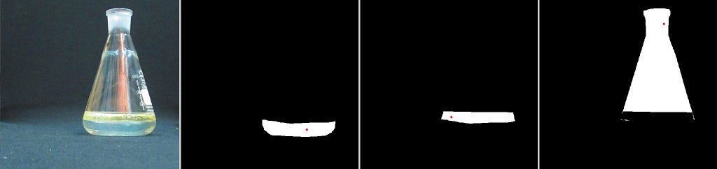
Now for the main function that will load the training batch. The training batch includes: One random image, all the segmentation masks belong to this image, and a random point in each mask:
def read_batch(data): # read random image and its annotaion from the dataset (LabPics)
# select image
ent = data[np.random.randint(len(data))] # choose random entry Img = cv2.imread(ent["image"])[...,::-1] # read image ann_map = cv2.imread(ent["annotation"]) # read annotation
inds = np.unique(mat_map)[1:] # load all indices points= [] masks = [] for ind in inds: mask=(mat_map == ind).astype(np.uint8) # make binary mask masks.append(mask) coords = np.argwhere(mask > 0) # get all coordinates in mask yx = np.array(coords[np.random.randint(len(coords))]) # choose random point/coordinate points.append([[yx[1], yx[0]]]) return Img,np.array(masks),np.array(points), np.ones([len(masks),1])
The first part of this function is choosing a random image and loading it:
ent  = data[np.random.randint(len(data))] # choose random entry
Img = cv2.imread(ent["image"])[...,::-1]  # read image
ann_map = cv2.imread(ent["annotation"]) # read annotation
Note that OpenCV reads images as BGR while SAM expects images as RGB, using […,::-1] to change the image from BGR to RGB.
Note that OpenCV reads images as BGR while SAM expects RGB images. By using […,::-1] we change the image from BGR to RGB.
SAM expects the image size to not exceed 1024, so we are going to resize the image and the annotation map to this size.
An important point here is that when resizing the annotation map (ann_map) we use INTER_NEAREST mode (nearest neighbors). In the annotation map, each pixel value is the index of the segment it belongs to. As a result, it’s important to use resizing methods that do not introduce new values to the map.
The next block is specific to the format of the LabPics1 dataset. The annotation map (ann_map) contains a segmentation map for the vessels in the image in one channel, and another map for the materials annotation in a different channel. We going to merge them into a single map.
What this gives us is a a map (mat_map) in which the value of each pixel is the index of the segment to which it belongs (for example: all cells with value 3 belong to segment 3). We want to transform this into a set of binary masks (0/1) where each mask corresponds to a different segment. In addition, from each mask, we want to extract a single point.
inds = np.unique(mat_map)[1:] # list of all indices in map
points= [] # list of all points (one for each mask)
masks = [] # list of all masks
for ind in inds:
            mask = (mat_map == ind).astype(np.uint8) # make binary mask for index ind
            masks.append(mask)
            coords = np.argwhere(mask > 0) # get all coordinates in mask
            yx = np.array(coords[np.random.randint(len(coords))]) # choose random point/coordinate
            points.append([[yx[1], yx[0]]])
return Img,np.array(masks),np.array(points), np.ones([len(masks),1])
This is it! We got the image (Img), a list of binary masks corresponding to segments in the image (masks), and for each mask the coordinate of a single point inside the mask (points).
Example for a batch of training data: 1) An Image. 2) List of segments masks. 3) For each mask a single point inside the mask (marked red for visualization only). Taken from the LabPics dataset.
Loading the SAM model
Now lets load the net:
sam2_checkpoint = "sam2_hiera_small.pt" # path to model weight
model_cfg = "sam2_hiera_s.yaml" # model config
sam2_model = build_sam2(model_cfg, sam2_checkpoint, device="cuda") # load model
predictor = SAM2ImagePredictor(sam2_model) # load net
First, we set the path to the model weights in: sam2_checkpoint parameter.We downloaded the weights earlier from here. “sam2_hiera_small.pt” refer to the small model but the code will work for any model you choose. Whichever model you choose you need to set the corresponding config file in the model_cfg parameter.The config files are already located in the sub folder“sam2_configs/” of the main repository.
Segment Anything General structure
Before setting training parameters we need to understand the basic structure of the SAM model.
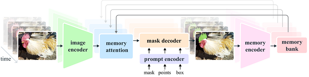
SAM is composed of three parts: 1) Image encoder, 2) Prompt encoder, 3) Mask decoder.
The image encoder is responsible for processing the image and creating the embedding that represents the image. This part consists of a VIT transformer and is the largest component of the net. We usually don’t want to train it, as it already gives good representation and training will demand lots of resources.
The prompt encoder processes the additional input to the net, in our case the input point.
The mask decoder takes the output of the image encoder and prompt encoder and produces the final segmentation masks. In general, we want to train only the mask decoder and maybe the prompt encoder. These parts are lightweight and can be fine-tuned fast with a modest GPU.
Setting training parameters:
We can enable the training of the mask decoder and prompt encoder by setting:
predictor.model.sam_mask_decoder.train(True) # enable training of mask decoder
predictor.model.sam_prompt_encoder.train(True) # enable training of prompt encoder
We also going to use mixed precision training which is just a more memory-efficient training strategy:
scaler = torch.cuda.amp.GradScaler() # set mixed precision
Main training loop
Now lets build the main training loop. The first part is reading and preparing the data:
for itr in range(100000):
    with torch.cuda.amp.autocast(): # cast to mix precision
            image,mask,input_point, input_label = read_batch(data) # load data batch
            if mask.shape[0]==0: continue # ignore empty batches
            predictor.set_image(image) # apply SAM image encoder to the image
First we cast the data to mix precision for efficient training:
with torch.cuda.amp.autocast():
Next, we use the reader function we created earlier to read training data:
Note that in this part we can also input boxes or masks but we are not going to use these options.
Now that we encoded both the prompt (points) and the image we can finally predict the segmentation masks:
batched_mode = unnorm_coords.shape[0] > 1 # multi mask prediction
high_res_features = [feat_level[-1].unsqueeze(0) for feat_level in predictor._features["high_res_feats"]]
low_res_masks, prd_scores, _, _ = predictor.model.sam_mask_decoder(image_embeddings=predictor._features["image_embed"][-1].unsqueeze(0),image_pe=predictor.model.sam_prompt_encoder.get_dense_pe(),sparse_prompt_embeddings=sparse_embeddings,dense_prompt_embeddings=dense_embeddings,multimask_output=True,repeat_image=batched_mode,high_res_features=high_res_features,)
prd_masks = predictor._transforms.postprocess_masks(low_res_masks, predictor._orig_hw[-1])# Upscale the masks to the original image resolution
The main part in this code is themodel.sam_mask_decoderwhich runs the mask_decoder part of the net and generates the segmentation masks (low_res_masks) and their scores (prd_scores).
These masks are in lower resolution than the original input image and are resized to the original input size in the postprocess_masksfunction.
This gives us the final prediction of the net: 3 segmentation masks (prd_masks) for each input point we used and the masks scores (prd_scores). prd_masks contains 3 predicted masks for each input point but we only going to use the first mask for each point. prd_scores contains a score of how good the net thinks each mask is (or how sure it is in the prediction).
Loss functions
Segmentation loss
Now we have the net predictions we can calculate the loss. First, we calculate the segmentation loss, which means how good the predicted mask is compared to the ground true mask. For this, we use the standard cross entropy loss.
First we need to convert prediction masks (prd_mask) from logits into probabilities using the sigmoid function:
prd_mask = torch.sigmoid(prd_masks[:, 0])# Turn logit map to probability map
Next we convert the ground truth mask into a torch tensor:
prd_mask = torch.sigmoid(prd_masks[:, 0])# Turn logit map to probability map
Finally, we calculate the cross entropy loss (seg_loss) manually using the ground truth (gt_mask) and predicted probability maps (prd_mask):
(we add 0.0001 to prevent the log function from exploding for zero values).
Score loss (optional)
In addition to the masks, the net also predicts the score for how good each predicted mask is. Training this part is less important but can be useful . To train this part we need to first know what is the true score of each predicted mask. Meaning, how good the predicted mask actually is. We are going to do it by comparing the GT mask and the corresponding predicted mask using intersection over union (IOU) metrics. IOU is simply the overlap between the two masks, divided by the combined area of the two masks. First, we calculate the intersection between the predicted and GT mask (the area in which they overlap):
inter = (gt_mask * (prd_mask > 0.5)).sum(1).sum(1)
We use threshold (prd_mask > 0.5) to turn the prediction mask from probability to binary mask.
Next, we get the IOU by dividing the intersection by the combined area (union) of the predicted and gt masks:
We going to use the IOU as the true score for each mask, and get the score loss as the absolute difference between the predicted scores and the IOU we just calculated.
And that it, we have trained/ fine-tuned the Segment-Anything 2 in less than 60 lines of code (not including comments and imports). After about 25,000 steps you should see major improvement .
First, we load the dependencies and cast the weights to float16 this makes the model much faster to run (only possible for inference).
import numpy as np
import torch
import cv2
from sam2.build_sam import build_sam2
from sam2.sam2_image_predictor import SAM2ImagePredictor

# use bfloat16 for the entire script (memory efficient)
torch.autocast(device_type="cuda", dtype=torch.bfloat16).__enter__()
Next, we load a sample image and a mask of the image region we want to segment (download image/mask):
image_path = r"sample_image.jpg" # path to image mask_path = r"sample_mask.png" # path to mask, the mask will define the image region to segment def read_image(image_path, mask_path): # read and resize image and mask img = cv2.imread(image_path)[...,::-1] # read image as rgb mask = cv2.imread(mask_path,0) # mask of the region we want to segment
Sample 30 random points inside the region we want to segment:
num_samples = 30 # number of points/segment to sample
def get_points(mask,num_points): # Sample points inside the input mask
        points=[]
        for i in range(num_points):
            coords = np.argwhere(mask > 0)
            yx = np.array(coords[np.random.randint(len(coords))])
            points.append([[yx[1], yx[0]]])
        return np.array(points)
input_points = get_points(mask,num_samples)
Load the standard SAM model (same as in training)
# Load model you need to have pretrained model already made
sam2_checkpoint = "sam2_hiera_small.pt"
model_cfg = "sam2_hiera_s.yaml"
sam2_model = build_sam2(model_cfg, sam2_checkpoint, device="cuda")
predictor = SAM2ImagePredictor(sam2_model)
Next, Load the weights of the model we just trained (model.torch):
Run the fine-tuned model to predict a segmentation mask for every point we selected earlier:
with torch.no_grad(): # prevent the net from caclulate gradient (more efficient inference)
        predictor.set_image(image) # image encoder
        masks, scores, logits = predictor.predict(  # prompt encoder + mask decoder
            point_coords=input_points,
            point_labels=np.ones([input_points.shape[0],1])
        )
Now we have a list of predicted masks and their scores. We want to somehow stitch them into a single consistent segmentation map. However, many of the masks overlap and might be inconsistent with each other. The approach to stitching is simple:
First we will sort the predicted masks according to their predicted scores:
Next, we add the masks one by one (from high to low score) to the segmentation map. We only add a mask if it’s consistent with the masks that were previously added, which means only if the mask we want to add has less than 15% overlap with already occupied areas.
for i in range(shorted_masks.shape[0]):
    mask = shorted_masks[i]
    if (mask*occupancy_mask).sum()/mask.sum()>0.15: continue
    mask[occupancy_mask]=0
    seg_map[mask]=i+1
    occupancy_mask[mask]=1
And this is it.
seg_mask now contains the predicted segmentation map with different values for each segment and 0 for the background.
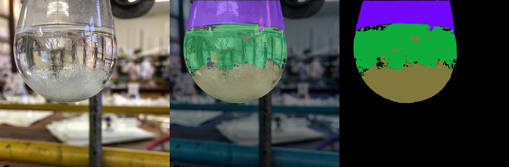
We can turn this into a color map using:
rgb_image = np.zeros((seg_map.shape[0], seg_map.shape[1], 3), dtype=np.uint8)
for id_class in range(1,seg_map.max()+1):
    rgb_image[seg_map == id_class] = [np.random.randint(255), np.random.randint(255), np.random.randint(255)]
That’s it, we have trained and tested SAM2 on a custom dataset. Other than changing the data-reader, this should work for any dataset. In many cases, this should be enough to give a significant improvement in performance.
If this is not the case, there is more we can do: Since we only fine-tuned the final part of the net (mask-decoder) we gave it a limited capacity to learn. The main part of SAM2 is the image encoder. This is the bulk part of the net and fine-tuning it will take more data and a stronger GPU, but will give the net more room for improvement.
You can train this part by adding the command:
predictor.model.image_encoder.train(True)
Note that in this case, you will also need to scan the SAM2 code for “no_grad” commands and remove them (“ no_grad” blocks the gradient collection, which saves memory but prevents training).
Finally, SAM2 can also segment and track objects in videos, but fine-tuning this part is for another time.
Copyright: All images for the post are taken from the SAM2 GIT repository (under Apache license), and LabPics dataset (under MIT license). This tutorial code and nets are available under the Apache license.
Today, we are excited to announce that the Snowflake Arctic Instruct model is available through Amazon SageMaker JumpStart to deploy and run inference. In this post, we walk through how to discover and deploy the Snowflake Arctic Instruct model using SageMaker JumpStart, and provide example use cases with specific prompts.
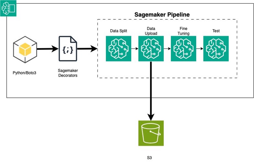
In this post, we show you how to convert Python code that fine-tunes a generative AI model in Amazon Bedrock from local files to a reusable workflow using Amazon SageMaker Pipelines decorators.
Today, divers recovered the body of tech entrepreneur Mike Lynch from the wreckage of his family’s superyacht Bayesian, which sunk off the coast of Sicily on Monday. Lynch — sometimes referred to as “Britain’s Bill Gates” — was holidaying in Sicily with his family and friends when disaster struck. An intense storm caused the Bayesian to capsize, plunging it to the bottom of the Mediterranean within minutes. Of the 22 people on board, seven died, including Lynch and his 18-year-old daughter Hannah. The tragedy comes just two months after a US jury found Lynch innocent of fraud charges in relation…
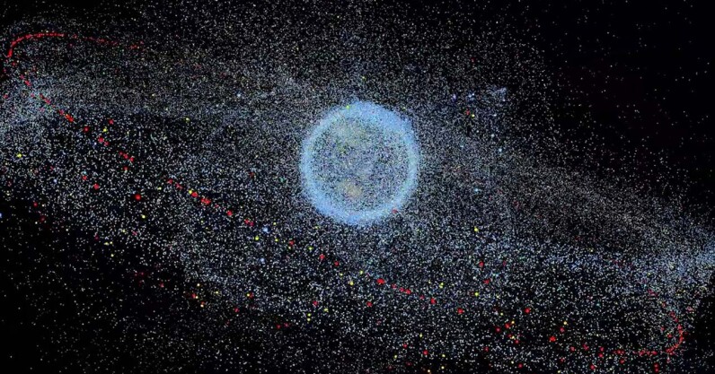
Space has become a crowded place. Astronomers estimate that over 10,000 active satellites were in orbit last month — four times as many as just five years ago. The surge in launches has ignited excitement about a new space race. But the cosmic traffic may be heading for a catastrophic crash. Back on Earth, the UK’s Space Operations Centre is tracking the threats with growing alarm. In July alone, the centre warned British satellite operators of 1,795 collision risks. Across the previous six months, almost 12,000 alerts were sent. Yet not every accident can be averted. In 2021, a Chinese military satellite was…
Apple Cash, a popular payment service, offers a seamless experience within the iOS Messages app. However, identity verification changes are coming for users.
Identity verification becomes mandatory for Apple Cash users in October
Starting October 4, 2024, Apple Cash will require users to verify their identity for certain transactions, marking a shift in the service’s operation.
Apple Cash users who have sent or received over $500, past or future, must verify their identity. The new rule applies to both new and past transactions.
We use cookies on our website to give you the most relevant experience by remembering your preferences and repeat visits. By clicking “Accept”, you consent to the use of ALL the cookies.
This website uses cookies to improve your experience while you navigate through the website. Out of these, the cookies that are categorized as necessary are stored on your browser as they are essential for the working of basic functionalities of the website. We also use third-party cookies that help us analyze and understand how you use this website. These cookies will be stored in your browser only with your consent. You also have the option to opt-out of these cookies. But opting out of some of these cookies may affect your browsing experience.
Necessary cookies are absolutely essential for the website to function properly. These cookies ensure basic functionalities and security features of the website, anonymously.
Cookie
Duration
Description
cookielawinfo-checkbox-analytics
11 months
This cookie is set by GDPR Cookie Consent plugin. The cookie is used to store the user consent for the cookies in the category "Analytics".
cookielawinfo-checkbox-functional
11 months
The cookie is set by GDPR cookie consent to record the user consent for the cookies in the category "Functional".
cookielawinfo-checkbox-necessary
11 months
This cookie is set by GDPR Cookie Consent plugin. The cookies is used to store the user consent for the cookies in the category "Necessary".
cookielawinfo-checkbox-others
11 months
This cookie is set by GDPR Cookie Consent plugin. The cookie is used to store the user consent for the cookies in the category "Other.
cookielawinfo-checkbox-performance
11 months
This cookie is set by GDPR Cookie Consent plugin. The cookie is used to store the user consent for the cookies in the category "Performance".
viewed_cookie_policy
11 months
The cookie is set by the GDPR Cookie Consent plugin and is used to store whether or not user has consented to the use of cookies. It does not store any personal data.
Functional cookies help to perform certain functionalities like sharing the content of the website on social media platforms, collect feedbacks, and other third-party features.
Performance cookies are used to understand and analyze the key performance indexes of the website which helps in delivering a better user experience for the visitors.
Analytical cookies are used to understand how visitors interact with the website. These cookies help provide information on metrics the number of visitors, bounce rate, traffic source, etc.
Advertisement cookies are used to provide visitors with relevant ads and marketing campaigns. These cookies track visitors across websites and collect information to provide customized ads.


