Dogecoin (DOGE) continued to demonstrate strength Tuesday following a crypto-market-wide resurgence led by Bitcoin. At press time, the top meme crypto was trading at $0.105, reflecting an impressive growth of just over 4% in the past 24 hours. Notably, this surge is partially being fueled by growing optimism around Dogecoin, with data from crypto analytics […]
The Binance ecosystem is on fire. The native coin, $BNB, is currently teetering between $574 and $575 and the ICO for the bep-20 store-of-value asset, Bitnance, has just passed 60,000 at presale. It appears 2024, could be a breakout end for Binance exchange, BNB Chain, and derivatives as the year ends. The $BNB coin is […]
Bitunix, a global crypto derivatives exchange, has announced a notable upgrade to its security following its partnership with Nemean Services, a UK-based digital asset security platform. According to an official release today, the exchange has received an additional $5 million in insurance coverage to further intensify its security for users’ assets. Bitunix Partners Renowned Leaders […]
Scaling reinforcement learning from tabular methods to large spaces
Reinforcement learning is a domain in machine learning that introduces the concept of an agent learning optimal strategies in complex environments. The agent learns from its actions, which result in rewards, based on the environment’s state. Reinforcement learning is a challenging topic and differs significantly from other areas of machine learning.
What is remarkable about reinforcement learning is that the same algorithms can be used to enable the agent adapt to completely different, unknown, and complex conditions.
Note. To fully understand the concepts included in this article, it is highly recommended to be familiar with concepts discussed in previous articles.
Up until now, we have only been discussing tabular reinforcement learning methods. In this context, the word “tabular” indicates that all possible actions and states can be listed. Therefore, the value function V or Q is represented in the form of a table, while the ultimate goal of our algorithms was to find that value function and use it to derive an optimal policy.
However, there are two major problems regarding tabular methods that we need to address. We will first look at them and then introduce a novel approach to overcome these obstacles.
This article is based on Chapter 9 of the book “Reinforcement Learning”written by Richard S. Sutton and Andrew G. Barto. I highly appreciate the efforts of the authors who contributed to the publication of this book.
1. Computation
The first aspect that has to be clear is that tabular methods are only applicable to problems with a small number of states and actions. Let us recall a blackjack example where we applied the Monte Carlo method in part 3. Despite the fact that there were only 200 states and 2 actions, we got good approximations only after executing several million episodes!
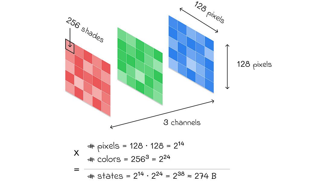
Imagine what colossal computations we would need to perform if we had a more complex problem. For example, if we were dealing with RGB images of size 128 × 128, then the total number of states would be 3 ⋅ 256 ⋅ 256 ⋅ 128 ⋅ 128 ≈ 274 billion. Even with modern technological advancements, it would be absolutely impossible to perform the necessary computations to find the value function!
Number of all possible states among 256 x 256 images.
In reality, most environments in reinforcement learning problems have a huge number of states and possible actions that can be taken. Consequently, value function estimation with tabular methods is no longer applicable.
2. Generalization
Even if we imagine that there are no problems regarding computations, we are still likely to encounter states that are never visited by the agent. How can standard tabular methods evaluate v- or q-values for such states?
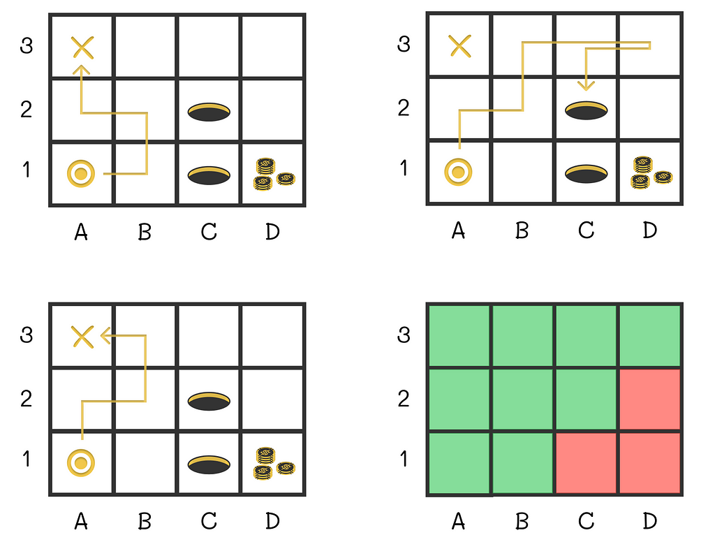
Images of the trajectories made by the agent in the maze during 3 different episodes. The bottom right image shows whether the agent has visited a given cell at least once (green color) or not (red color). For unvisited states, standard tabular methods cannot obtain any information.
This article will propose a novel approach based on supervised learning that will efficiently approximate value functions regardless the number of states and actions.
Idea
The idea of value-function approximation lies in using a parameterized vector w that can approximate a value function. Therefore, from now on, we will write the value function v̂ as a function of two arguments: state s and vector w:
Our objective is to find v̂ and w. The function v̂ can take various forms but the most common approach is to use a supervised learning algorithm. As it turns out, v̂ can be a linear regression, decision tree, or even a neural network. At the same time, any state s can be represented as a set of features describing this state. These features serve as an input for the algorithm v̂.
Why are supervised learning algorithms used for v̂?
It is known that supervised learning algorithms are very good at generalization. In other words, if a subset (X₁, y₁) of a given dataset D for training, then the model is expected to also perform well for unseen examples X₂.
At the same time, we highlighted above the generalization problem for reinforcement learning algorithms. In this scenario, if we apply a supervised learning algorithm, then we should no longer worry about generalization: even if a model has not seen a state, it would still try to generate a good approximate value for it using available features of the state.
Example
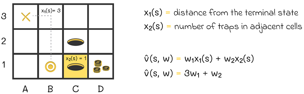
Let us return to the maze and show an example of how the value function can look. We will represent the current state of the agent by a vector consisting of two components:
x₁(s) is the distance between the agent and the terminal state;
x₂(s) is the number of traps located around the agent.
For v, we can use the scalar product of s and w. Assuming that the agent is currently located at cell B1, the value function v̂ will take the form shown in the image below:
An example of the scalar product used to represent the state value function. The agent’s state is represented by two features. The distance from the agent’s position (B1) to the terminal state (A3) is 3. Adjacent trap cell (C1), with the respect to the current agent’s position, is colored in yellow.
Difficulties
With the presented idea of supervised learning, there are two principal difficulties we have to address:
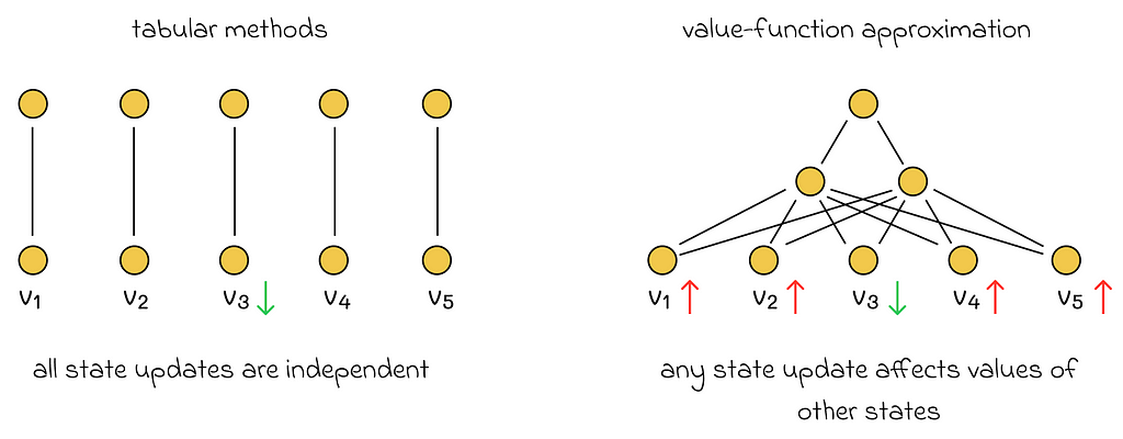
1. Learned state values are no longer decoupled. In all previous algorithms we discussed, an update of a single state did not affect any other states. However, now state values depend on vector w. If the vector w is updated during the learning process, then it will change the values of all other states. Therefore, if w is adjusted to improve the estimate of the current state, then it is likely that estimations of other states will become worse.
The difference between updates in tabular and value-function approximation methods. In the image, the state value v3 is updated. Green arrows show a decrease in the resulting errors in value state approximations, while red arrows represent the error increase.
2. Supervised learning algorithms require targets for training that are not available. We want a supervised algorithm to learn the mapping between states and true value functions. The problem is that we do not have any true state values. In this case, it is not even clear how to calculate a loss function.
The prediction objective
State distribution
We cannot completely get rid of the first problem, but what we can do is to specify how much each state is important to us. This can be done by creating a state distribution that maps every state to its importance weight.
This information can then be taken into account in the loss function.
Most of the time, μ(s) is chosen proportionally to how often state s is visited by the agent.
Loss function
Assuming that v̂(s, w) is differentiable, we are free to choose any loss function we like. Throughout this article, we will be looking at the example of the MSE (mean squared error). Apart from that, to account for the state distribution μ(s), every error term is scaled by its corresponding weight:
In the shown formula, we do not know the true state values v(s). Nevertheless, we will be able to overcome this issue in the next section.
Objective
After having defined the loss function, our ultimate goal becomes to find the best vector w that will minimize the objective VE(w). Ideally, we would like to converge to the global optimum, but in reality, the most complex algorithms can guarantee convergence only to a local optimum. In other words, they can find the best vector w* only in some neighbourhood of w.
Despite this fact, in many practical cases, convergence to a local optimum is often enough.
Stochastic-gradient methods
Stochastic-gradient methods are among the most popular methods to perform function approximation in reinforcement learning.
Let us assume that on iteration t, we run the algorithm through a single state example. If we denote by wₜ a weight vector at step t, then using the MSE loss function defined above, we can derive the update rule:
We know how to update the weight vector w but what can we use as a target in the formula above? First of all, we will change the notation a little bit. Since we cannot obtain exact true values, instead of v(S), we are going to use another letter U, which will indicate that true state values are approximated.
The ways the state values can be approximated are discussed in the following sections.
Gradient Monte Carlo
Monte Carlo is the simplest method that can be used to approximate true values. What makes it great is that the state values computed by Monte Carlo are unbiased! In other words, if we run the Monte Carlo algorithm for a given environment an infinite number of times, then the averaged computed state values will converge to the true state values:
Why do we care about unbiased estimations? According to theory, if target values are unbiased, then SGD is guaranteed to converge to a local optimum (under appropriate learning rate conditions).
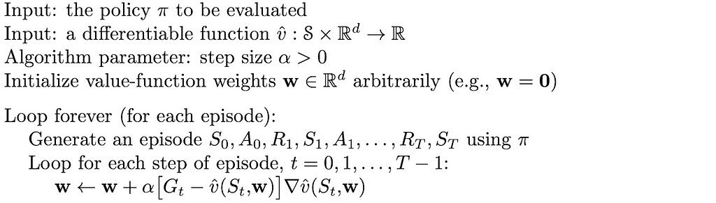
In this way, we can derive the Gradient Monte Carlo algorithm, which uses expected returns Gₜ as values for Uₜ:
Once the whole episode is generated, all expected returns are computed for every state included in the episode. The respective expected returns are used during the weight vector w update. For the next episode, new expected returns will be calculated and used for the update.
As in the original Monte Carlo method, to perform an update, we have to wait until the end of the episode, and that can be a problem in some situations. To overcome this disadvantage, we have to explore other methods.
Bootstrapping
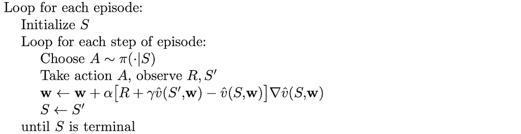
At first sight, bootstrapping seems like a natural alternative to gradient Monte Carlo. In this version, every target is calculated using the transition reward R and the target value of the next state (or n steps later in the general case):
However, there are still several difficulties that need to be addressed:
Bootstrapped values are biased. At the beginning of an episode, state values v̂ and weights w are randomly initialized. So it is an obvious fact that on average, the expected value of Uₜ will not approximate true state values. As a consequence, we lose the guarantee of converging to a local optimum.
Target values depend on the weight vector. This aspect is not typical in supervised learning algorithms and can create complications when performing SGD updates. As a result, we no longer have the opportunity to calculate gradient values that would lead to the loss function minimization, according to the classical SGD theory.
The good news is that both of these problems can be overcome with semi-gradient methods.
Semi-gradient methods
Despite losing important convergence guarantees, it turns out that using bootstrapping under certain constraints on the value function (discussed in the next section) can still lead to good results.
As we have already seen in part 5, compared to Monte Carlo methods, bootstrapping offers faster learning, enabling it to be online and is usually preferred in practice. Logically, these advantages also hold for gradient methods.
Linear methods
Let us look at a particular case where the value function is a scalar product of the weight vector w and the feature vector x(s):
The choice of the linear function is particularly attractive because, from the mathematical point of view, value approximation problems become much easier to analyze.
Instead of the SGD algorithm, it is also possible to use the method of least squares.
Linear function in gradient Monte Carlo
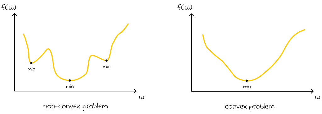
The choice of the linear function makes the optimization problem convex. Therefore, there is only one optimum.
Convex problems have only one local minimum, which is the global optimum.
In this case, regarding gradient Monte Carlo (if its learning rate αis adjusted appropriately), an important conclusion can be made:
Since the gradient Monte Carlo method is guaranteed to converge to a local optimum, it is automatically guaranteed that the found local optimum will be global when using the linear value approximation function.
Linear function in semi-gradient methods
According to theory, under the linear value function, gradient one-step TD algorithms also converge. The only subtlety is that the convergence point (which is called the TD fixed point) is usually located near the global optimum. Despite this, the approximation quality with the TD fixed point if often enough in most tasks.
Conclusion
In this article, we have understood the scalability limitations of standard tabular algorithms. This led us to the exploration of value-function approximation methods. They allow us to view the problem from a slightly different angle, which elegantly transforms the reinforcement learning problem into a supervised machine learning task.
The previous knowledge of Monte Carlo and bootstrapping methods helped us elaborate their respective gradient versions. While gradient Monte Carlo comes with stronger theoretical guarantees, bootstrapping (especially the one-step TD algorithm) is still a preferred method due to its faster convergence.
Graph RAG answers the big questions where text embeddings won’t help you.
Retrieval Augmented Generation (RAG) has dominated the discussion around making Gen AI applications useful since ChatGPT’s advent exploded the AI hype. The idea is simple. LLMs become especially useful once we connect them to our private data. A foundational model, that everyone has access to, combined with our domain-specific data as the secret sauce results in a potent, unique tool. Just like in the human world, AI systems seem to develop into an economy of experts. General knowledge is a useful base, but expert knowledge will work out your AI system’s unique selling proposition.
Recap: RAG itself does not yet describe any specific architecture or method. It only depicts the augmentation of a given generation task with an arbitrary retrieval method. The original RAG paper (Retrieval-Augmented Generation for Knowledge-Intensive NLP Tasks by Lewis et. al.) compares a two-tower embedding approach with bag-of-words retrieval.
Local and Global Questions
Text Embedding-based retrieval has been described in many occurrences. It already allows our LLM application to answer questions based on the content of a given knowledge base extremely reliably. The core strength of Text2Vec retrieval remains: Extracting a given fact represented in the embedded knowledge base and formulating an answer to the user query that is grounded using that extracted fact. However, text embedding search also comes with major challenges. Usually, every text embedding represents one specific chunk from the unstructured dataset. The nearest neighbor search finds embeddings that represent chunks semantically similar to the incoming user query. That also means the search is semantic but still highly specific. Thus candidate quality is highly dependent on query quality. Furthermore, embeddings represent the content mentioned in your knowledge base. This does not represent cases in which you are looking to answer questions that require an abstraction across documents or concepts within a document in your knowledge base.
For example, imagine a knowledge base containing the bios of all past Nobel Peace Prize winners. Asking the Text2Vec-RAG system “Who won the Nobel Peace Prize 2023?” would be an easy question to answer. This fact is well represented in the embedded document chunks. Thus the final answer can be grounded in the correct context. On the other hand, the RAG system might struggle by asking “Who were the most notable Nobel Peace Prize winners of the last decade?”. We might be successful after adding more context such as “Who were the most notable Nobel Peace Prize winners fighting against the Middle East conflict?”, but even that will be a difficult one to solve solely based on text embeddings (given the current quality of embedding models). Another example is whole dataset reasoning. For example, your user might be interested in asking your LLM application “What are the top 3 topics that recent Nobel Peace Prize winners stood up for?”. Embedded chunks do not allow reasoning across documents. Our nearest neighbor search is looking for a specific mention of “the top 3 topics that recent Nobel Peace Prize winners stood up for” in the knowledge base. If this is not included in the knowledge base, any purely text-embedding-based LLM application will struggle and most likely fail to answer this question correctly and especially exhaustively.
We need an alternative retrieval method that allows us to answer these “Global”, aggregative questions in addition to the “Local” extractive questions. Welcome to Graph RAG!
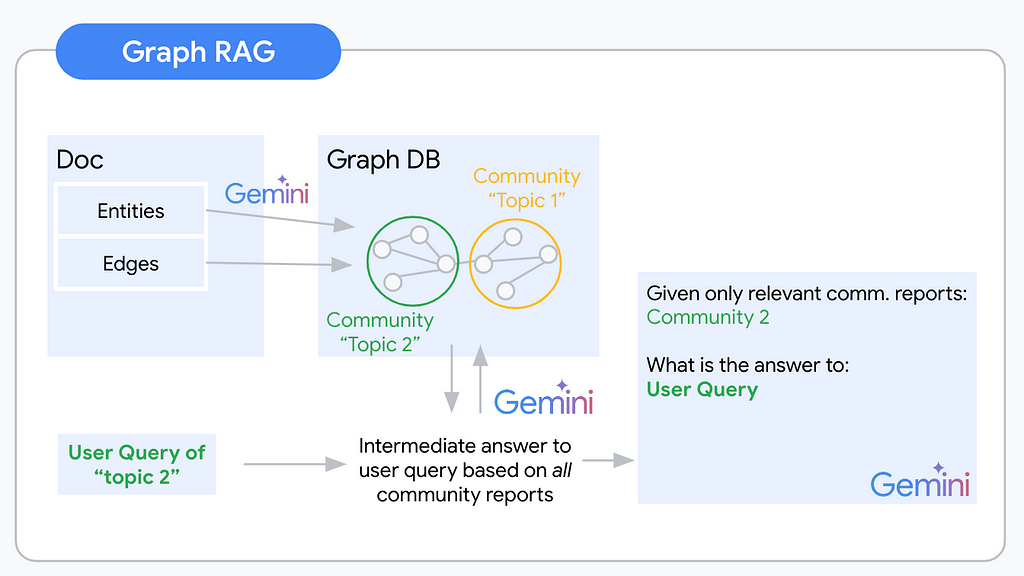
Knowledge Graphs are a semi-structured, hierarchical approach to organizing information. Once information is organized as a graph we can infer information about specific nodes, but also their relationships and neighbors. The graph structure allows reasoning on a global dataset level because nodes and the connections between them can span across documents. Given this graph, we can also analyze neighboring nodes and communities of nodes that are more tightly connected within each other than they are to other nodes. A community of nodes can be expected to roughly cover one topic of interest. Abstracting across the community nodes and their connections can give us an abstract understanding of concepts within this topic. Graph RAG uses this understanding of communities within a knowledge graph to propose context for a given user query.
A Graph RAG pipeline will usually follow the following steps:
Graph Extraction
Graph Storage
Community detection
Community report generation
Map Reduce for final context building
GraphRAG Logic Visualized — Source: Image by the author
Graph Extraction
The process of building abstracted understanding for our unstructured knowledge base begins with extracting the nodes and edges that will build your knowledge graph. You automate this extraction via an LLM. The biggest challenge of this step is deciding which concepts and relationships are relevant to include. To give an example for this highly ambiguous task: Imagine you are extracting a knowledge graph from a document about Warren Buffet. You could extract his holdings, place of birth, and many other facts as entities with respective edges. Most likely these will be highly relevant information for your users. (With the right document) you could also extract the color of his tie at the last board meeting. This will (most likely) be irrelevant to your users. It is crucial to specify the extraction prompt to the application use case and domain. This is because the prompt will determine what information is extracted from the unstructured data. For example, if you are interested in extracting information about people, you will need to use a different prompt than if you are interested in extracting information about companies.
The easiest way to specify the extraction prompt is via multishot prompting. This involves giving the LLM multiple examples of the desired input and output. For instance, you could give the LLM a series of documents about people and ask it to extract the name, age, and occupation of each person. The LLM would then learn to extract this information from new documents. A more advanced way to specify the extraction prompt is through LLM fine-tuning. This involves training the LLM on a dataset of examples of the desired input and output. This can cause better performance than multishot prompting, but it is also more time-consuming.
You designed a solid extraction prompt and tuned your LLM. Your extraction pipeline works. Next, you will have to think about storing these results. Graph databases (DB) such as Neo4j and Arango DB are the straightforward choice. However, extending your tech stack by another db type and learning a new query language (e.g. Cypher/Gremlin) can be time-consuming. From my high-level research, there are also no great serverless options available. If handling the complexity of most Graph DBs was not enough, this last one is a killer for a serverless lover like myself. There are alternatives though. With a little creativity for the right data model, graph data can be formatted as semi-structured, even strictly structured data. To get you inspired I coded up graph2nosql as an easy Python interface to store and access your graph dataset in your favorite NoSQL db.
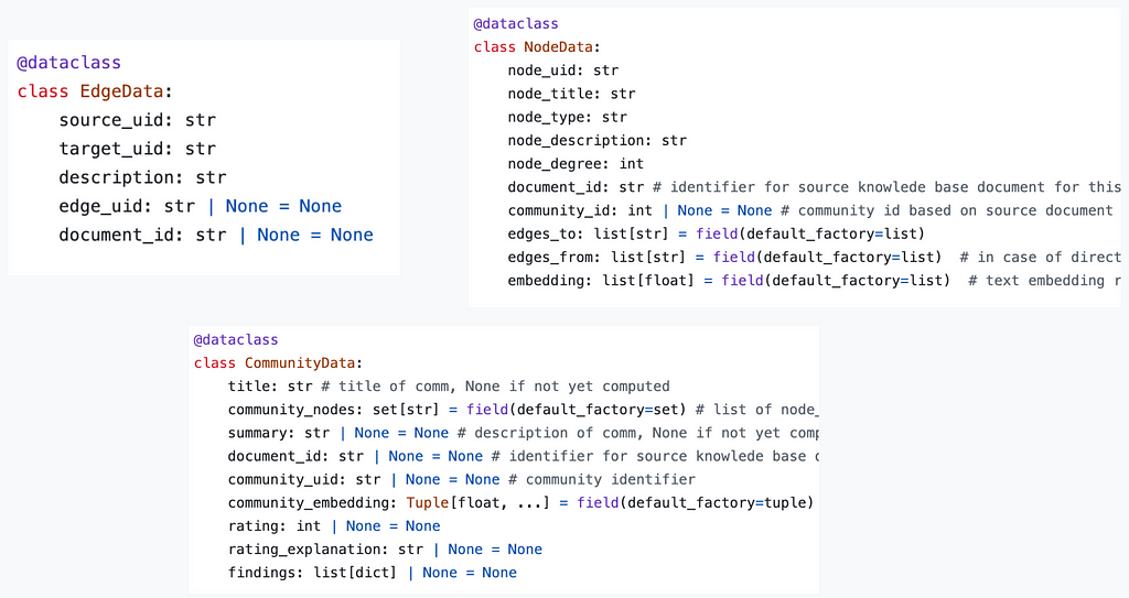
The data model defines a format for Nodes, Edges, and Communities. Store all three in separate collections. Every node, edge, and community finally identify via a unique identifier (UID). Graph2nosql then implements a couple of essential operations needed when working with knowledge graphs such as adding/removing nodes/edges, visualizing the graph, detecting communities, and more.
graph2nosql data model — Source: Image by the author
Community Detection
Once the graph is extracted and stored, the next step is to identify communities within the graph. Communities are clusters of nodes that are more tightly connected than they are to other nodes in the graph. This can be done using various community detection algorithms.
One popular community detection algorithm is the Louvain algorithm. The Louvain algorithm works by iteratively merging nodes into communities until a certain stopping criterion is met. The stopping criterion is typically based on the modularity of the graph. Modularity is a measure of how well the graph is divided into communities.
Other popular community detection algorithms include:
Girvan-Newman Algorithm
Fast Unfolding Algorithm
Infomap Algorithm
Community Report Generation
Now use the resulting communities as a base to generate your community reports. Community reports are summaries of the nodes and edges within each community. These reports can be used to understand graph structure and identify key topics and concepts within the knowledge base. In a knowledge graph, every community can be understood to represent one “topic”. Thus every community might be a useful context to answer a different type of questions.
Aside from summarizing multiple nodes’ information, community reports are the first abstraction level across concepts and documents. One community can span over the nodes added by multiple documents. That way you’re building a “global” understanding of the indexed knowledge base. For example, from your Nobel Peace Prize winner dataset, you probably extracted a community that represents all nodes of the type “Person” that are connected to the node “Nobel Peace prize” with the edge description “winner”.
A great idea from the Microsoft Graph RAG implementation are “findings”. On top of the general community summary, these findings are more detailed insights about the community. For example, for the community containing all past Nobel Peace Prize winners, one finding could be some of the topics that connected most of their activism.
Just as with graph extraction, community report generation quality will be highly dependent on the level of domain and use case adaptation. To create more accurate community reports, use multishot prompting or LLM fine-tuning.
At query time you use a map-reduce pattern to first generate intermediate responses and a final response.
In the map step, you combine every community-userquery pair and generate an answer to the user query using the given community report. In addition to this intermediate response to the user question, you ask the LLM to evaluate the relevance of the given community report as context for the user query.
In the reduce step you then order the relevance scores of the generated intermediate responses. The top k relevance scores represent the communities of interest to answer the user query. The respective community reports, potentially combined with the node and edge information are the context for your final LLM prompt.
Closing thoughts: Where is this going?
Text2vec RAG leaves obvious gaps when it comes to knowledge base Q&A tasks. Graph RAG can close these gaps and it can do so well! The additional abstraction layer via community report generation adds significant insights into your knowledge base and builds a global understanding of its semantic content. This will save teams an immense amount of time screening documents for specific pieces of information. If you are building an LLM application it will enable your users to ask the big questions that matter. Your LLM application will suddenly be able to seemingly think around the corner and understand what is going on in your user’s data instead of “only” quoting from it.
On the other hand, a Graph RAG pipeline (in its raw form as described here) requires significantly more LLM calls than a text2vec RAG pipeline. Especially the generation of community reports and intermediate answers are potential weak points that are going to cost a lot in terms of dollars and latency.
As so often in search you can expect the industry around advanced RAG systems to move towards a hybrid approach. Using the right tool for a specific query will be essential when it comes to scaling up RAG applications. A classification layer to separate incoming local and global queries could for example be imaginable. Maybe the community report and findings generation is enough and adding these reports as abstracted knowledge into your index as context candidates suffices.
Luckily the perfect RAG pipeline is not solved yet and your experiments will be part of the solution. I would love to hear about how that is going for you!
In this post, we provide an overview of Amazon Q Business Confluence Cloud connector and how you can use it for seamless integration of generative AI assistance to your Confluence Cloud.
Bungie has finally brought all of the “Marathon” trilogy of games to Steam, with “Marathon Infinity” now playable for free on modern Macs.
Marathon Infinite [Bungie, macOS]
In May, Bungie started to bring Marathon to Steam, with the intention of bringing all three titles to the digital storefront as free releases. On Thursday, Bungie concluded the trilogy.
Classic Marathon Infinity is a free game on the Steam storefront, playable on both Mac and Windows PC. It is a faithful re-release of the 1995 first-person shooter, using the original data files, but modernized.
Classic ‘Marathon Infinity’ lands on Steam as a free Mac title
Originally appeared here:
Classic ‘Marathon Infinity’ lands on Steam as a free Mac title
We use cookies on our website to give you the most relevant experience by remembering your preferences and repeat visits. By clicking “Accept”, you consent to the use of ALL the cookies.
This website uses cookies to improve your experience while you navigate through the website. Out of these, the cookies that are categorized as necessary are stored on your browser as they are essential for the working of basic functionalities of the website. We also use third-party cookies that help us analyze and understand how you use this website. These cookies will be stored in your browser only with your consent. You also have the option to opt-out of these cookies. But opting out of some of these cookies may affect your browsing experience.
Necessary cookies are absolutely essential for the website to function properly. These cookies ensure basic functionalities and security features of the website, anonymously.
Cookie
Duration
Description
cookielawinfo-checkbox-analytics
11 months
This cookie is set by GDPR Cookie Consent plugin. The cookie is used to store the user consent for the cookies in the category "Analytics".
cookielawinfo-checkbox-functional
11 months
The cookie is set by GDPR cookie consent to record the user consent for the cookies in the category "Functional".
cookielawinfo-checkbox-necessary
11 months
This cookie is set by GDPR Cookie Consent plugin. The cookies is used to store the user consent for the cookies in the category "Necessary".
cookielawinfo-checkbox-others
11 months
This cookie is set by GDPR Cookie Consent plugin. The cookie is used to store the user consent for the cookies in the category "Other.
cookielawinfo-checkbox-performance
11 months
This cookie is set by GDPR Cookie Consent plugin. The cookie is used to store the user consent for the cookies in the category "Performance".
viewed_cookie_policy
11 months
The cookie is set by the GDPR Cookie Consent plugin and is used to store whether or not user has consented to the use of cookies. It does not store any personal data.
Functional cookies help to perform certain functionalities like sharing the content of the website on social media platforms, collect feedbacks, and other third-party features.
Performance cookies are used to understand and analyze the key performance indexes of the website which helps in delivering a better user experience for the visitors.
Analytical cookies are used to understand how visitors interact with the website. These cookies help provide information on metrics the number of visitors, bounce rate, traffic source, etc.
Advertisement cookies are used to provide visitors with relevant ads and marketing campaigns. These cookies track visitors across websites and collect information to provide customized ads.