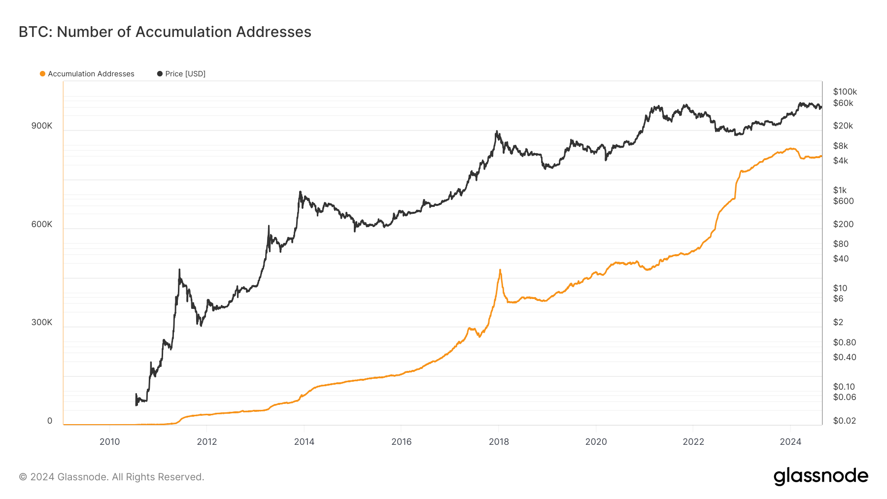
Onchain Highlights DEFINITION: The number of unique accumulation addresses. Accumulation addresses are defined as addresses that have at least 2 incoming non-dust transfers and have never spent funds. Exchange addresses and addresses receiving from coinbase transactions (miner addresses) are discarded. To account for lost coins, addresses that were last active more than 7 years ago are […]
The influx of institutional demand has likely been one of the major factors that explained why Bitcoin hovered around the previous cycle ATHs.
Investors need not fear lower timeframe volatility
SOL has been trading sideways lately after being one of the year’s most volatile cryptos
Worth looking at if and how the Solana network’s slowdown contributed to SOL’s current situation
Justin Sun downplayed risk USDD fears after withdrawing its 12K BTC collateral.
Despite the reassurance, an analyst viewed Sun as a likely risk factor in the space.
Harris aide believes the VP’s crypto-policies will support emerging technologies
Execs like Coinbase’s Chief Policy Officer reacted positively to this outreach effort
After reading this article, you’ll be very well equipped with the tools and reasoning capability to think about the effects of any Lk regularization term and decide if it applies to your situation.
What is regularization in machine learning?
Let’s look at some definitions on the internet and generalize based on those.
Regularization is a set of methods for reducing overfitting in machine learning models. Typically, regularization trades a marginal decrease in training accuracy for an increase in generalizability. (IBM)
Regularization makes models stable across different subsets of the data. It reduces the sensitivity of model outputs to minor changes in the training set. (geeksforgeeks)
Regularization in machine learning serves as a method to forestall a model from overfitting. (simplilearn)
In general, regularization is a technique to prevent the model from overfitting and to allow the model to generalize its predictions on unseen data. Let’s look at the role of weight regularization in particular.
Why use weight regularization?
One could employ many forms of regularization while training a machine learning model. Weight regularization is one such technique, which is the focus of this article. Weight regularization means applying some constraints on the learnable weights of your machine learning model so that they allow the model to generalize to unseen inputs.
Weight regularization improves the performance of neural networks by penalizing the weight matrices of nodes. This penalty discourages the model from having large parameter (weight) values. It helps control the model’s ability to fit the noise in the training data. Typically, the biases in the machine learning model are not subject to regularization.
How is regularization implemented in deep neural networks?
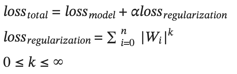
Typically, a regularization loss is added to the model’s loss during training. It allows us to control the model’s weights during training. The formula looks like this:
Figure-1: Total loss as a sum of the model loss and regularization loss. k is a floating point value and indicates the regularization norm. Alpha is the weighting factor for the regularization loss.
Typical values of k used in practice are 1 and 2. These are called the L1 and L2 regularization schemes.
But why do we use just these two values for the most part, when in fact there are infinitely many values of k one could use? Let’s answer this question with an interpretation of the L1 and L2 regularization schemes.
Interpretation of different weight regularization types
The two most common types of regularization used for machine learning models are L1 and L2 regularization. We will start with these two, and continue to discuss some unusual regularization types such as L0.5 and L3 regularization. We will take a look at the gradients of the regularization losses and plot them to intuitively understand how they affect the model weights.
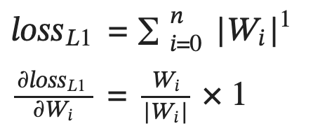
L1 regularization
L1 regularization adds the average of the absolute value of the weights together as the regularization loss.
Figure-2: L1 regularization loss and its partial derivative with respect to each weight Wi.
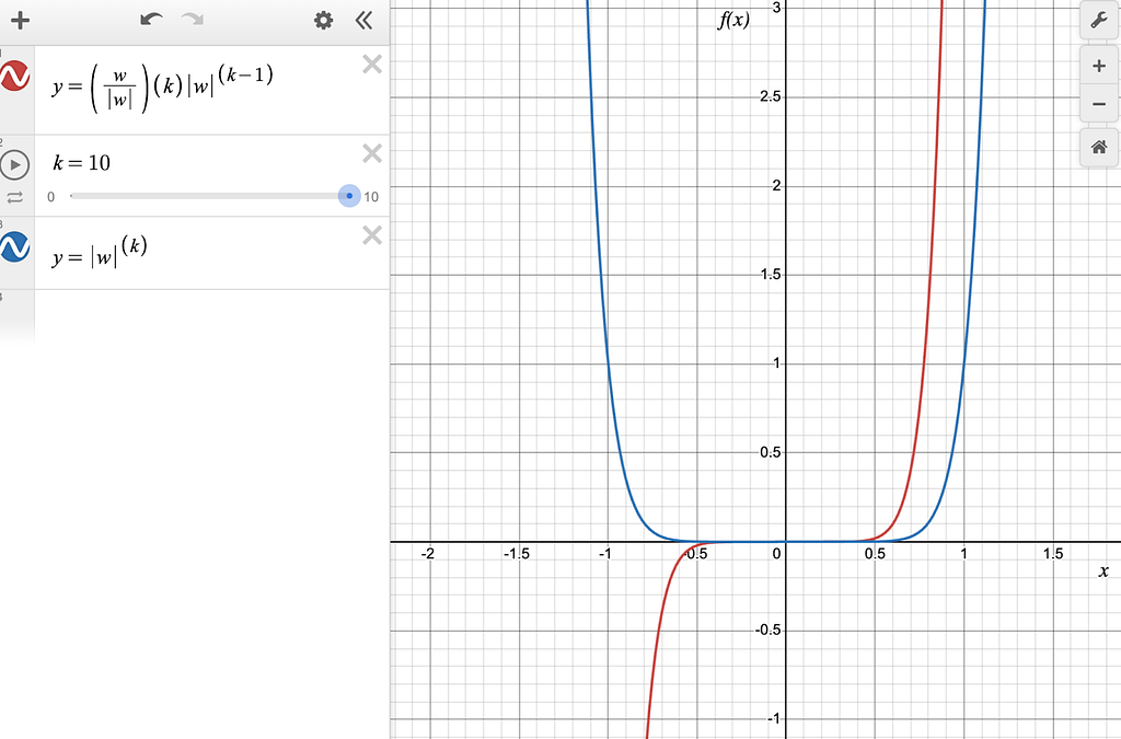
It has the effect of adjusting the weights by a constant (in this case alpha times the learning rate) in the direction that minimizes the loss. Figure 3 shows a graphical representation of the function and its derivative.
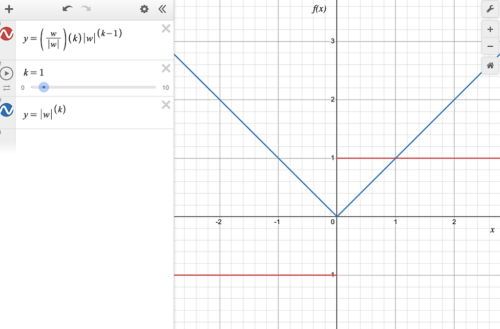
Figure-3: The blue line is |w| and the red line is the derivative of |w|.
You can see that the derivative of the L1 norm is a constant (depending on the sign of w), which means that the gradient of this function only depends on the sign of w and not its magnitude. The gradient of the L1 norm is not defined at w=0.
It means that the weights are moved towards zero by a constant value at each step during backpropagation. Throughout training, it has the effect of driving the weights to converge at zero. That is why the L1 regularization makes a model sparse (i.e. some of the weights become 0). It might cause a problem in some cases if it ends up making a model too sparse. The L2 regularization does not have this side-effect. Let’s discuss it in the next section.
L2 regularization
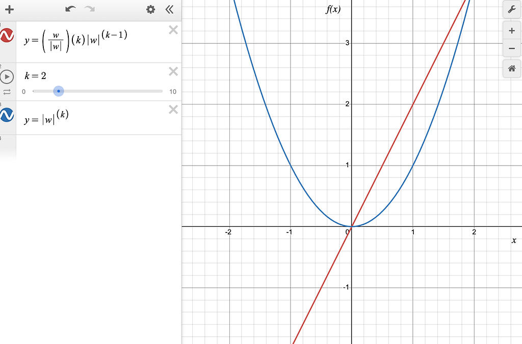
L2 regularization adds the average of the square of the absolute value of the weights together as the regularization loss.
Figure-4: L2 regularization loss and its partial derivative with respect to each weight Wi.
It has the effect of adjusting each weight by a multiple of the weight itself in the direction that minimizes the loss. Figure 5 shows a graphical representation of the function and its derivative.
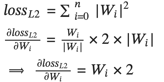
Figure-5: The blue line is pow(|w|, 2) and the red line is the derivative of pow(|w|, 2).
You can see that the derivative of the L2 norm is just the sign-adjusted square root of the norm itself. The gradient of the L2 norm depends on both the sign and magnitude of the weight.
This means that at every gradient update step, the weights will be adjusted toward zero by an amount that is proportional to the weight’s value. Over time, this has the effect of drawing the weights toward zero, but never exactly zero, since subtracting a constant factor of a value from the value itself never makes the result exactly zero unless it is zero to begin with. The L2 norm is commonly used for weight decay during machine learning model training.
Let’s consider L0.5 regularization next.
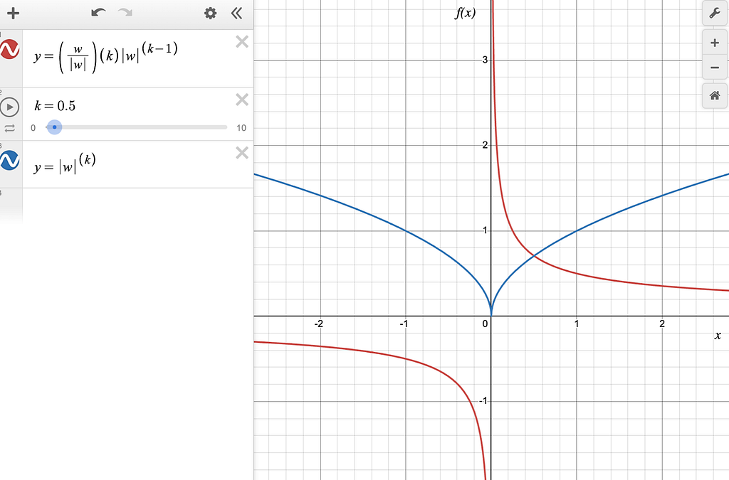
L0.5 regularization
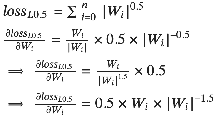
L0.5 regularization adds the average of the square root of the absolute value of the weights together as the regularization loss.
Figure-6: L0.5 regularization loss and its partial derivative with respect to each weight Wi.
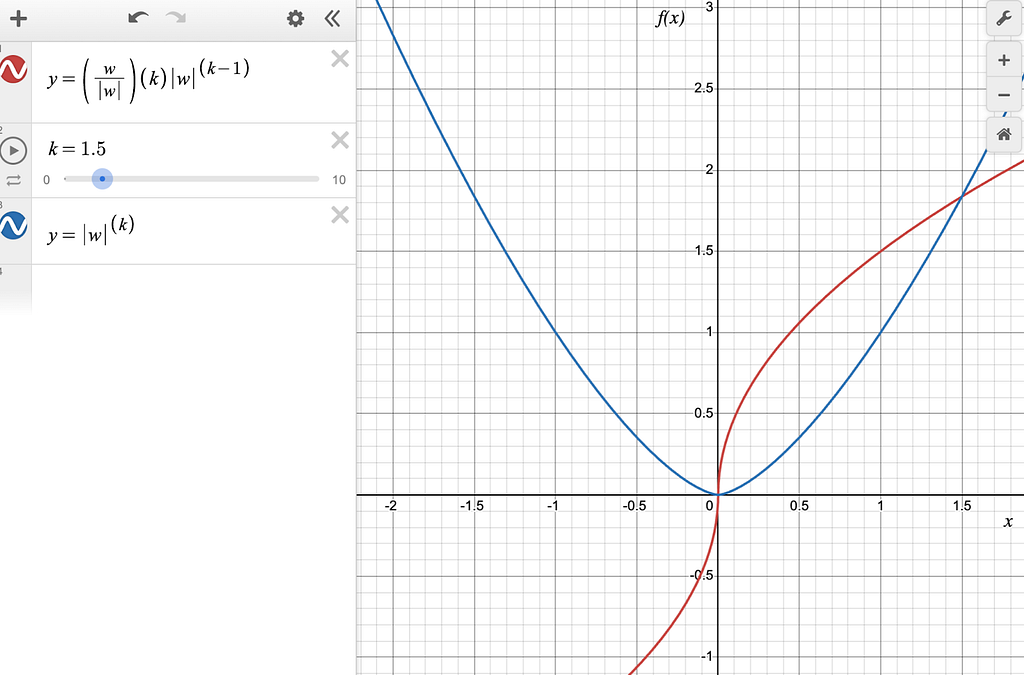
This has the effect of adjusting each weight by a multiple (in this case alpha times the learning rate) of the inverse square root of the weight itself in the direction that minimizes the loss. Figure 7 shows a graph of the function and its derivative.
Figure-7: The blue line is pow(|w|, 0.5) and the red line is the derivative of pow(|w|, 0.5).
You can see that the derivative of the L0.5 norm is a discontinuous function, which peaks at the positive values of w close to 0 and it reaches negative infinity for the negative values of w close to 0. Further, we can draw the following conclusions from the graph:
As |w| tends to 0, the magnitude of the gradient tends to infinity. During backpropagation, these values of w will quickly swing to past 0 because large gradients will cause a large change in the value of w. In other words, negative w will become positive and vice-versa. This cycle of flip flops will continue to repeat itself.
As |w| increases, the magnitude of the gradient decreases. These values of w are stable because of small gradients. However, with each backpropagation step, the value of w will be drawn closer to 0.
This is hardly what one would want from a weight regularization routine, so it’s safe to say that L0.5 isn’t a great weight regularizer. Let’s consider L3 regularization next.
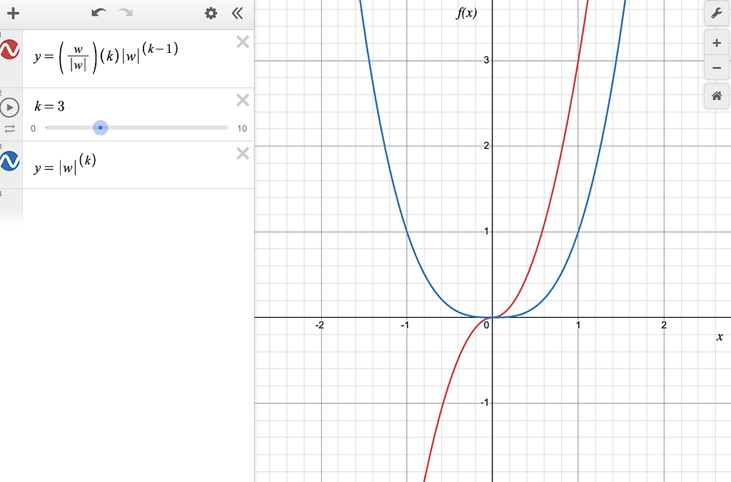
L3 regularization
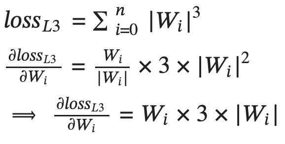
L3 regularization adds the average of the cube of the absolute value of the weights together as the regularization loss.
Figure-8: L3 regularization loss and its partial derivative with respect to each weight Wi.
This has the effect of adjusting each weight by a multiple (in this case alpha times the learning rate) of the square of the weight itself in the direction that minimizes the loss.
Graphically, this is what the function and its derivative look like.
Figure-9: The blue line is pow(|w|, 3) and the red line is the derivative of pow(|w|, 3).
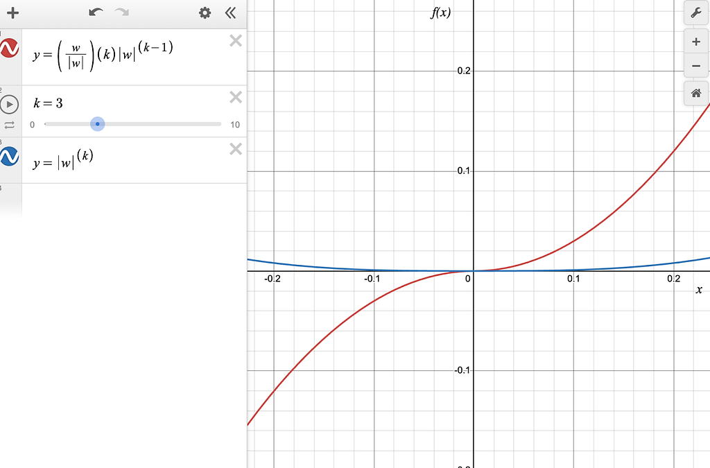
To really understand what’s going on here, we need to zoom in to the chart around the w=0 point.
Figure-10: The blue line is pow(|w|, 3) and the red line is the derivative of pow(|w|, 3), zoomed in at small values of w around 0.0.
You can see that the derivative of the L3 norm is a continuous and differentiable function (despite the presence of |w| in the derivative), which has a large magnitude at large values of w and a small magnitude for small values of w.
Interestingly, the gradient is very close to zero for very small values of w around the 0.0 mark.
The interpretation of the gradient for L3 is interesting.
For large values of w, the magnitude of the gradient is large. During backpropagation, these values will be pushed towards 0.
Once the weight w reaches an inflection point (close to 0.0), the gradient almost vanishes, and the weights will stop getting updated.
The effect is that it will drive the weights with large magnitudes close to 0, but not exactly 0.
Let’s consider higher norms to see how this plays out in the limiting case.
Beyond L3 regularization
To understand what happens for Linfinity, we need to see what happens in the case of the L10 regularization case.
Figure-11: The blue line is pow(|w|, 10) and the red line is the derivative of pow(|w|, 10), zoomed in at small values of w around 0.0.
One can see that the gradients for values of |w| < 0.5 are extremely small, which means that regularization won’t be effective for those values of w.
Exercise
Based on everything we saw above, L1 and L2 regularization are fairly practical based on what you want to achieve. As an exercise, try to reason about the behavior of the L1.5 regularization, whose chart is shown below.
Figure-12: The blue line is pow(|w|, 1.5) and the red line is the derivative of pow(|w|, 1.5).
Conclusion
We took a visual and intuitive look at the L1 and L2 (and in general Lk) regularization terms to understand why L1 regularization results in sparse model weights and L2 regularization results in model weights close to 0. Framing the solution as inspecting the resulting gradients is extremely valuable during this exercise.
We explored L0.5, L3, and L10 regularization terms and graphically, and you (the reader) reasoned about regularization terms between L1 and L2 regularization, and developed an intuitive understanding of what implications it would have on a model’s weights.
We hope that this article has added to your toolbox of tricks you can use when considering regularization strategies during model training to fine-tuning.
All the charts in this article were created using the online desmos graphing calculator. Here is a link to the functions used in case you wish to play with them.
All the images were created by the author(s) unless otherwise mentioned.
References
We found the following articles useful while researching the topic, and we hope that you find them useful too!
We use cookies on our website to give you the most relevant experience by remembering your preferences and repeat visits. By clicking “Accept”, you consent to the use of ALL the cookies.
This website uses cookies to improve your experience while you navigate through the website. Out of these, the cookies that are categorized as necessary are stored on your browser as they are essential for the working of basic functionalities of the website. We also use third-party cookies that help us analyze and understand how you use this website. These cookies will be stored in your browser only with your consent. You also have the option to opt-out of these cookies. But opting out of some of these cookies may affect your browsing experience.
Necessary cookies are absolutely essential for the website to function properly. These cookies ensure basic functionalities and security features of the website, anonymously.
Cookie
Duration
Description
cookielawinfo-checkbox-analytics
11 months
This cookie is set by GDPR Cookie Consent plugin. The cookie is used to store the user consent for the cookies in the category "Analytics".
cookielawinfo-checkbox-functional
11 months
The cookie is set by GDPR cookie consent to record the user consent for the cookies in the category "Functional".
cookielawinfo-checkbox-necessary
11 months
This cookie is set by GDPR Cookie Consent plugin. The cookies is used to store the user consent for the cookies in the category "Necessary".
cookielawinfo-checkbox-others
11 months
This cookie is set by GDPR Cookie Consent plugin. The cookie is used to store the user consent for the cookies in the category "Other.
cookielawinfo-checkbox-performance
11 months
This cookie is set by GDPR Cookie Consent plugin. The cookie is used to store the user consent for the cookies in the category "Performance".
viewed_cookie_policy
11 months
The cookie is set by the GDPR Cookie Consent plugin and is used to store whether or not user has consented to the use of cookies. It does not store any personal data.
Functional cookies help to perform certain functionalities like sharing the content of the website on social media platforms, collect feedbacks, and other third-party features.
Performance cookies are used to understand and analyze the key performance indexes of the website which helps in delivering a better user experience for the visitors.
Analytical cookies are used to understand how visitors interact with the website. These cookies help provide information on metrics the number of visitors, bounce rate, traffic source, etc.
Advertisement cookies are used to provide visitors with relevant ads and marketing campaigns. These cookies track visitors across websites and collect information to provide customized ads.