Blog

A quick-start tutorial

The landscape of artificial intelligence (AI), particularly in Generative AI, has seen significant advancements recently. Large Language Models (LLMs) have been truly transformative in this regard. One popular approach to building an LLM application is Retrieval Augmented Generation (RAG), which combines the ability to leverage an organization’s data with the generative capabilities of these LLMs. Agents are a popular and useful way to introduce autonomous behaviour into LLM applications.

What is Agentic RAG?

Agentic RAG represents an advanced evolution in AI systems, where autonomous agents utilize RAG techniques to enhance their decision-making and response abilities. Unlike traditional RAG models, which often rely on user input to trigger actions, agentic RAG systems adopt a proactive approach. These agents autonomously seek out relevant information, analyse it and use it to generate responses or take specific actions. An agent is equipped with a set of tools and can judiciously select and use the appropriate tools for the given problem.

This proactive behaviour is particularly valuable in many use cases such as customer service, research assistance, and complex problem-solving scenarios. By integrating the generative capability of LLMs with advanced retrieval systems agentic RAG offers a much more effective AI solution.

Key Features of RAG Using Agents

1.Task Decomposition:

Agents can break down complex tasks into manageable subtasks, handling retrieval and generation step-by-step. This approach enhances the coherence and relevance of the final output.

2. Contextual Awareness:

RAG agents maintain contextual awareness throughout interactions, ensuring that retrieved information aligns with the ongoing conversation or task. This leads to more coherent and contextually appropriate responses.

3. Flexible Retrieval Strategies:

Agents can adapt their retrieval strategies based on the context, such as switching between dense and sparse retrieval or employing hybrid approaches. This optimization balances relevance and speed.

4. Feedback Loops:

Agents often incorporate mechanisms to use user feedback for refining future retrievals and generations, which is crucial for applications that require continuous learning and adaptation.

5. Multi-Modal Capabilities:

Advanced RAG agents are starting to support multi-modal capabilities, handling and generating content across various media types (text, images, videos). This versatility is useful for diverse use cases.

6. Scalability:

The agent architecture enables RAG systems to scale efficiently, managing large-scale retrievals while maintaining content quality, making them suitable for enterprise-level applications.

7.Explainability:

Some RAG agents are designed to provide explanations for their decisions, particularly in high-stakes applications, enhancing trust and transparency in the system’s outputs.

This blog post is a getting-started tutorial which guides the user through building an agentic RAG system using Langchain with IBM Watsonx.ai (both for embedding and generative capabilities) and Milvus vector database service provided through IBM Watsonx.data (for storing the vectorized knowledge chunks). For this tutorial, we have created a ReAct agent.

Step 1: Package installation

Let us first install the necessary Python packages. These include Langchain, IBM Watson integrations, milvus integration packages, and BeautifulSoup4 for web scraping.

%pip install langchain
%pip install langchain_ibm
%pip install BeautifulSoup4
%pip install langchain_community
%pip install langgraph
%pip install pymilvus
%pip install langchain_milvus

Step 2: Imports

Next we import the required libraries to set up the environment and configure our LLM.

import bs4
from Langchain.tools.retriever import create_retriever_tool
from Langchain_community.document_loaders import WebBaseLoader
from Langchain_core.chat_history import BaseChatMessageHistory
from Langchain_core.prompts import ChatPromptTemplate
from Langchain_text_splitters import CharacterTextSplitter
from pymilvus import MilvusClient, DataType
import os, re

Here, we are importing modules for web scraping, chat history, text splitting, and vector storage (milvus)

Step 3: Configuring environment variables

We need to set up environment variables for IBM Watsonx, which will be used to access the LLM which is provided by Watsonx.ai

os.environ["WATSONX_APIKEY"] = "<Your_API_Key>"
os.environ["PROJECT_ID"] = "<Your_Project_ID>"
os.environ["GRPC_DNS_RESOLVER"] = "<Your_DNS_Resolver>"

Please make sure to replace the placeholder values with your actual credentials.

Step 4: Initializing Watsonx LLM

With the environment set up, we initialize the IBM Watsonx LLM with specific parameters to control the generation process. We are using the ChatWatsonx class here with mistralai/mixtral-8x7b-instruct-v01 model from watsonx.ai.

from Langchain_ibm import ChatWatsonx

llm = ChatWatsonx(
    model_id="mistralai/mixtral-8x7b-instruct-v01",
    url="https://us-south.ml.cloud.ibm.com",
    project_id=os.getenv("PROJECT_ID"),
    params={
            "decoding_method": "sample",
            "max_new_tokens": 5879,
            "min_new_tokens": 2,
            "temperature": 0,
            "top_k": 50,
            "top_p": 1,
        }
)

This configuration sets up the LLM for text generation. We can tweak the inference parameters here for generating desired responses. More information about model inference parameters and their permissible values here

Step 5: Loading and splitting documents

We load the documents from a web page and split them into chunks to facilitate efficient retrieval. The chunks generated are stored in the milvus instance that we have provisioned.

loader = WebBaseLoader(
    web_paths=("https://lilianweng.github.io/posts/2023-06-23-agent/",),
    bs_kwargs=dict(
        parse_only=bs4.SoupStrainer(
            class_=("post-content", "post-title", "post-header")
        )
    ),
)
docs = loader.load()
text_splitter = CharacterTextSplitter(chunk_size=1500, chunk_overlap=200)
splits = text_splitter.split_documents(docs)

This code scrapes content from a specified web page, then splits the content into smaller segments, which will later be indexed for retrieval.

Disclaimer: We have confirmed that this site allows scraping, but it’s important to always double-check the site’s permissions before scraping. Websites can update their policies, so ensure your actions comply with their terms of use and relevant laws.

Step 6: Setting up the retriever

We establish a connection to Milvus to store the document embeddings and enable fast retrieval.

from AdpativeClient import InMemoryMilvusStrategy, RemoteMilvusStrategy, BasicRAGHandler

def adapt(number_of_files=0, total_file_size=0, data_size_in_kbs=0.0):
    strategy = InMemoryMilvusStrategy()
    if(number_of_files > 10 or total_file_size > 10 or data_size_in_kbs > 0.25):
        strategy = RemoteMilvusStrategy()
    client = strategy.connect()
    return client

client = adapt(total_size_kb)
handler = BasicRAGHandler(client)
retriever = handler.create_index(splits)

This function decides whether to use an in-memory or remote Milvus instance based on the size of the data, ensuring scalability and efficiency.

BasicRAGHandler class covers the following functionalities at a high level:

· Initializes the handler with a Milvus client, allowing interaction with the Milvus vector database provisioned through IBM Watsonx.data

· Generates document embeddings, defines a schema, and creates an index in Milvus for efficient retrieval.

· Inserts document, their embeddings and metadata into a collection in Milvus.

Step 7: Defining the tools

With the retrieval system set up, we now define retriever as a tool . This tool will be used by the LLM to perform context-based information retrieval

tool = create_retriever_tool(
    retriever,
    "blog_post_retriever",
    "Searches and returns excerpts from the Autonomous Agents blog post.",
)
tools = [tool]

Step 8: Generating responses

Finally, we can now generate responses to user queries, leveraging the retrieved content.

from langgraph.prebuilt import create_react_agent
from Langchain_core.messages import HumanMessage

agent_executor = create_react_agent(llm, tools)

response = agent_executor.invoke({"messages": [HumanMessage(content="What is ReAct?")]})
raw_content = response["messages"][1].content

In this tutorial (link to code), we have demonstrated how to build a sample Agentic RAG system using Langchain and IBM Watsonx. Agentic RAG systems mark a significant advancement in AI, combining the generative power of LLMs with the precision of sophisticated retrieval techniques. Their ability to autonomously provide contextually relevant and accurate information makes them increasingly valuable across various domains.

As the demand for more intelligent and interactive AI solutions continues to rise, mastering the integration of LLMs with retrieval tools will be essential. This approach not only enhances the accuracy of AI responses but also creates a more dynamic and user-centric interaction, paving the way for the next generation of AI-powered applications.

NOTE: This content is not affiliated with or endorsed by IBM and is in no way an official IBM documentation. It is a personal project pursued out of personal interest, and the information is shared to benefit the community.

Building an Agentic Retrieval-Augmented Generation (RAG) System with IBM Watsonx and Langchain was originally published in Towards Data Science on Medium, where people are continuing the conversation by highlighting and responding to this story.

How can we improve observability with open-source tools?

Traditional monitoring no longer meets the needs of complex data organizations. Instead of relying on reactive systems to identify known issues, data engineers must create interactive observability frameworks that help them quickly find any type of anomaly.

While observability can encompass many different practices, in this article, I’ll share a high-level overview and practical tips from our experience building an observability framework in our organization using open-source tools.

So, how to build infrastructure that has good data health visibility and ensures data quality?

What is data observability?

Overall, observability defines how much you can tell about an internal system from its external outputs. The term was first defined in 1960 by Hungarian-American engineer Rudolf E. Kálmán, who discussed observability in mathematical control systems.

Over the years, the concept has been adapted to various fields, including data engineering. Here, it addresses the issue of data quality and being able to track where the data was gathered and how it was transformed.

Data observability means ensuring that data in all pipelines and systems is integral and of high quality. This is done by monitoring and managing real-time data to troubleshoot quality concerns. Observability assures clarity, which allows action before the problem spreads.

What is a data observability framework?

Data observability framework is a process of monitoring and validating data integrity and quality within an institution. It helps to proactively ensure data quality and integrity.

The framework must be based on five mandatory aspects, as defined by IBM:

1. Freshness. Outdated data, if any, must be found and removed.
2. Distribution. Expected data values must be recorded to help identify outliers and unreliable data.
3. Volume. The number of expected values must be tracked to ensure data is complete.
4. Schema. Changes to data tables and organization must be monitored to help find broken data.
5. Lineage. Collecting metadata and mapping the sources is a must to aid troubleshooting.

These five principles ensure that data observability frameworks help maintain and increase data quality. You can achieve these by implementing the following data observability methods.

How to add observability practices into the data pipeline

Only high-quality data collected from reputable sources will provide precise insights. As the saying goes: garbage in, garbage out. You cannot expect to extract any actual knowledge from poorly organized datasets.

As a senior data analyst at public data provider Coresignal, I constantly seek to find new ways to improve data quality. While it’s quite a complex goal to achieve in the dynamic tech landscape, many paths lead to it. Good data observability plays an important role here.

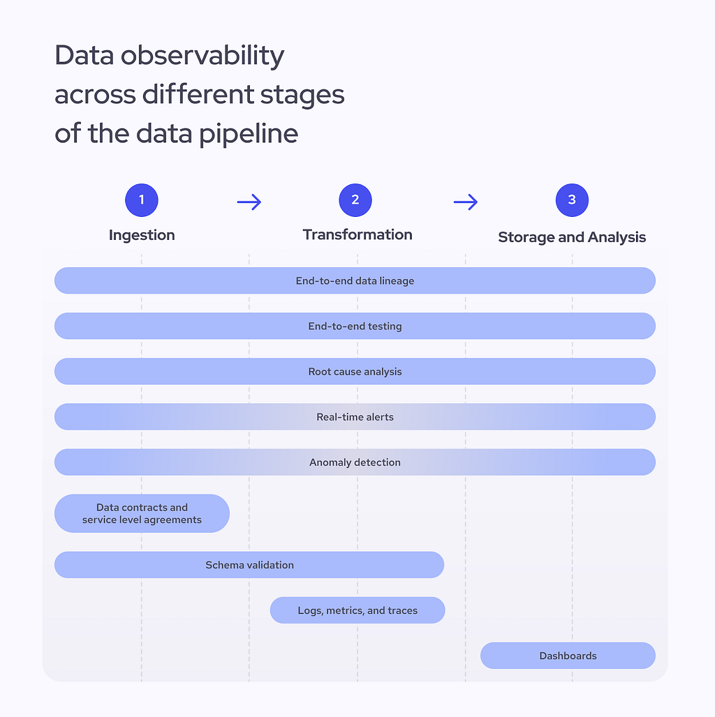
So, how do we ensure the quality of data? It all comes down to adding better observability methods into each data pipeline stage — from ingestion and transformation to storage and analysis. Some of these methods will work across the entire pipeline while others will be relevant in only one stage of it. Let’s take a look:

First off, we have to consider five items that cover the entire pipeline:

1. End-to-end data lineage. Tracking lineage lets you quickly access database history and follow your data from the original source to the final output. By understanding the structure and its relationships, you will have less trouble finding inconsistencies before they become problems.
2. End-to-end testing. A validation process that checks data integrity and quality at each data pipeline stage helps engineers determine if the pipeline functions correctly and spot any untypical behaviors.
3. Root cause analysis. If issues emerge at any stage of the pipeline, engineers must be able to pinpoint the source precisely and find a quick solution.
4. Real-time alerts. One of the most important observability goals is to quickly spot emerging issues. Time is of the essence when flagging abnormal behaviors, so any data observability framework has to be able to send alerts in real time. This is especially important for the data ingestion as well as storage and analysis phases.
5. Anomaly detection. Issues such as missing data or low performance can happen anywhere across the data pipeline. Anomaly detection is an advanced observability method that is likely to be implemented later in the process. In most cases, machine learning algorithms will be required to detect unusual patterns in your data and logs.

Then, we have five other items that will be more relevant in one data pipeline stage than the other:

1. Service level agreements (SLAs). SLAs help set standards for the client and the supplier and define the data quality, integrity, and general responsibilities. SLA thresholds can also help when setting up an alert system, and typically, they will be signed before or during the ingestion phase.
2. Data contracts. These agreements define how data is structured before it enters other systems. They act as a set of rules that clarify what level of freshness and quality you can expect and will usually be negotiated before the ingestion phase.
3. Schema validation. It guarantees consistent data structures and ensures compatibility with downstream systems. Engineers usually validate the schema during the ingestion or processing stages.
4. Logs, metrics, and traces. While essential for monitoring performance, collecting and easily accessing this crucial information will become a helpful tool in a crisis — it allows one to find the root cause of a problem faster.
5. Data quality dashboards. Dashboards help monitor the overall health of the data pipeline and have a high-level view of possible problems. They ensure that the data gathered using other observability methods is presented clearly and in real time.

Finally, data observability cannot be implemented without adding self-evaluation to the framework, so constant auditing and reviewing of the system is a must for any organization.

Next, let’s discuss the tools you might want to try to make your work easier.

Data observability platforms and what can you do with them

So, which tools should you consider if you are beginning to build a data observability framework in your organization? While there are many options out there, in my experience, your best bet would be to start out with the following tools.

As we were building our data infrastructure, we focused on making the most out of open source platforms. The tools listed below ensure transparency and scalability while working with large amounts of data. While most of them have other purposes than data observability, combined, they provide a great way to ensure visibility into the data pipeline.

Here is a list of five necessary platforms that I would recommend to check out:

1. Prometheus and Grafana platforms complement each other and help engineers collect and visualize large amounts of data in real time. Prometheus, an open-source monitoring system, is perfect for data storage and observation, while the observability platform Grafana helps track new trends through an easy-to-navigate visual dashboard.
2. Apache Iceberg table format provides an overview of database metadata, including tracking statistics about table columns. Tracking metadata helps to better understand the entire database without unnecessarily processing it. It’s not exactly an observability platform, but its functionalities allow engineers to get better visibility into their data.
3. Apache Superset is another open-source data exploration and visualization tool that can help to present huge amounts of data, build dashboards, and generate alerts.
4. Great Expectations is a Python package that helps test and validate data. For instance, it can scan a sample dataset using predefined rules and create data quality conditions that are later used for the entire dataset. Our teams use Great Expectations to run quality tests on new datasets.
5. Dagster data pipeline orchestration tool can help ensure data lineage and run asset checks. While it was not created as a data observability platform, it provides visibility using your existing data engineering tools and table formats. The tool aids in figuring out the root causes of data anomalies. The paid version of the platform also contains AI-generated insights. This application provides self-service observability and comes with an in-built asset catalog for tracking data assets.

Keep in mind that these are just some of the many options available. Make sure to do your research and find the tools that make sense for your organization.

What happens if you ignore the data observability principles

Once a problem arises, organizations usually rely on an engineer’s intuition to find the root cause of the problem. As software engineer Charity Majors vividly explains in her recollection of her time at MBaaS platform Parse, most traditional monitoring is powered by engineers who have been at the company the longest and can quickly guess their system’s issues. This makes senior engineers irreplaceable and creates additional issues, such as high rates of burnout.

Using data observability tools eliminates guesswork from troubleshooting, minimizes the downtime, and enhances trust. Without data observability tools, you can expect high downtime, data quality issues, and slow reaction times to emerging issues. As a result, these problems might quickly lead to loss of revenue, customers, or even damage brand reputation.

Data observability is vital for enterprise-level companies that handle gargantuan amounts of information and must guarantee its quality and integrity without interruptions.

What’s next for data observability?

Data observability is a must for every organization, especially companies that work with data collection and storage. Once all the tools are set in place, it’s possible to start using advanced methods to optimize the process.

Machine learning, especially large language models (LLMs), is the obvious solution here. They can help to quickly scan the database, flag anomalies, and help to improve the overall data quality by spotting duplicates or adding new enriched fields. At the same time, these algorithms can help keep track of the changes in the schema and logs, improving the data consistency and improving data lineage.

However, it is crucial to pick the right time to implement your AI initiatives. Enhancing your observability capabilities requires resources, time, and investment. Before starting to use custom LLMs, you should carefully consider whether this would truly benefit your organization. Sometimes, it might be more efficient to stick to the standard open-source data observability tools listed above, which are already effective in getting the job done.

Building a Robust Data Observability Framework to Ensure Data Quality and Integrity was originally published in Towards Data Science on Medium, where people are continuing the conversation by highlighting and responding to this story.

A powerful yet under-the-radar method for data summarization and explainable AI

Despite being a powerful tool for data summarization, the MMD-Critic method has a surprising lack of both usage and “coverage”. Perhaps this is because simpler and more established methods for data summarization exist (e.g. K-medoids, see [1] or, more simply, the Wikipedia page), or perhaps this is because no Python package for the method existed (before now). Regardless, the results presented in the original paper [2] warrant more use than MMD-Critic has currently. As such, I’ll explain the MMD-Critic method here with as much clarity as possible. I’ve also published an open-source Python package with an implementation of the technique so you can use it easily.

Prototypes and Criticisms

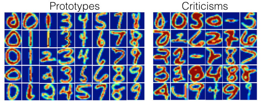
Before jumping into the MMD-Critic method itself, it’s worth discussing what exactly we’re trying to accomplish. Ultimately, we wish to take a dataset and find examples that are representative of the data (prototypes), as well as edge-case examples that may confound our machine learning models (criticisms).

There are many reasons why this may be useful:

• We can get a very nice summarized view of our dataset by seeing both stereotypical and atypical examples
• We can test models on the criticisms to see how they handle edge cases (this is, for obvious reasons, very important)
• Though perhaps not as useful, we can use prototypes to create a naturally explainable K-means-esque algorithm wherein the closest prototype to the new data point is used to label it. Then explanations are simple since we just show the user the most similar data point.
• More

You can see section 6.3 in this book for more info on the applications of this (and for a decent explanation of MMD-Critic as well), but it suffices to say that finding these examples is useful for a wide variety of reasons. MMD-Critic allows us to do this.

Maximal Mean Discrepancy

I unfortunately cannot claim to have a hyper-rigorous understanding of Maximal Mean Discrepancy (MMD), as such an understanding would require a strong background in functional analysis. If you have such a background, you can find the paper that introduced the measure here.

In simple terms though, MMD is a way to determine the difference between two probability distributions. Formally, for two probability distributions P and Q, we define the MMD of the two as

Here, F is any function space — that is, any set of functions with the same domain and codomain. Note also that the notation x~P means that we are treating x as if it’s a random variable drawn from the distribution P — that is, x is described by P. This formula thus finds the highest difference in the expected values of X and Y when they are transformed by some function from our space F.

This may be a little hard to wrap your head around, but here’s an example. Suppose that X is Uniform(0, 1) (i.e. a distribution that is equivalent to picking a random number from 0 to 1), and Y is Uniform(-1, 1) . Let’s also let F be a fairly simple family containing three functions — f(x) = 0, f(x) = x, and f(x) = x². Iterating over each function in our space, we get:

1. In the f(x) = 0 case, E[f(x)] when x ~ P is 0 since no matter what x we choose, f(x) will be 0. The same holds for when x ~ Q. Thus, we get a mean discrepancy of 0
2. In the f(x) = x case, we have E[f(x)] = 0.5 for the P case and 0 for the Q case, so our mean discrepancy is 0.5
3. In the f(x) = x² case, we note that

thus in the P case, we get

and in the Q case, we get

thus our discrepancy in this case is also 0. The supremum over our function space is thus 0.5, so that’s our MMD.

You may now notice a few problems with our MMD. It seems highly dependent on our choice of function space and also appears highly expensive (or even impossible) to compute for a large or infinite function space. Not only that, but it also requires us to know our distributions P and Q, which is not realistic.

The latter problem is easily solvable, as we can rewrite our MMD metric to use estimates of P and Q based on our dataset:

Here, our x’s are our samples from the dataset drawing from P, and the y’s are the samples drawn from Q.

The first two problems are solvable with a bit of extra math. Without going into too much detail, it turns out that if F is something called a Reproducing Kernel Hilbert Space (RKHS), we know what function is going to give us our MMD in advance. Namely, it’s the following function, called the witness function:

where k is the kernel (inner product) associated with the RKHS¹. Intuitively, this function “witnesses” the discrepancy between P and Q at the point x.

We thus only need to choose a sufficiently expressive RKHS/kernel — usually, the RBF kernel is used which has the kernel function

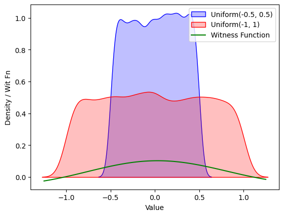
This generally gets fairly intuitive results. Here, for instance, is the plot of the witness function with the RBF kernel when estimated (in the same way as mentioned before — that is, replacing expectations with a sum) on two datasets drawn from Uniform(-0.5, 0.5) and Uniform(-1, 1) :

The code for generating the above graph is here:

import numpy as np
import matplotlib.pyplot as plt
import seaborn as sns

def rbf(v1, v2, sigma=0.5):
  return np.exp(-(v2 - v1) ** 2/(2 * sigma**0.5))

def comp_wit_fn(x, d1, d2):
  return 1/len(d1) * sum([rbf(x, dp) for dp in d1]) - 1/len(d2) * sum([rbf(x, dp) for dp in d2])

low1, high1 = -0.5, 0.5  # Range for the first uniform distribution
low2, high2 = -1, 1  # Range for the second uniform distribution

# Generate data for the uniform distributions
data1 = np.random.uniform(low1, high1, 10000)
data2 = np.random.uniform(low2, high2, 10000)

# Generate a range of x values for which to compute comp_wit_fn
x_values = np.linspace(min(low1 * 2, low2 * 2), max(high1 * 2, high2 * 2), 100)

comp_wit_values = [comp_wit_fn(x, data1, data2) for x in x_values]
sns.kdeplot(data1, label=f'Uniform({low1}, {high1})', color='blue', fill=True)
sns.kdeplot(data2, label=f'Uniform({low2}, {high2})', color='red', fill=True)
plt.plot(x_values, comp_wit_values, label='Witness Function', color='green')

plt.xlabel('Value')
plt.ylabel('Density / Wit Fn')
plt.legend()
plt.show()

The MMD-Critic Method, Finally

The idea behind MMD-Critic is now fairly simple — if we want to find k prototypes, we need to find the set of prototypes that best matches the distribution of the original dataset given by their squared MMD. In other words, we wish to find a subset P of cardinality k of our dataset that minimizes MMD²(F, X, P). Without going into too much detail about why, the square MMD is given by

After finding these prototypes, we then select the points where the hypothetical distribution of our prototypes is most different from our dataset distribution as criticisms. As we’ve seen before, the difference between two distributions at a point can be measured by our witness function, so we just find points that maximize its absolute value in the context of X and P. In other words, we define our criticism “score” as

Or, in the more usable approximate form,

Then, to find our desired amount of criticisms, say m of them, we simply wish to find the set C of size m that maximizes

To promote picking more varied criticisms, the paper also suggests adding a regularizer term that encourages selected criticisms to be as far apart as possible. The suggested regularizer in the paper is the log determinant regularizer, though this is not required. I won’t go into much detail here since it’s not critical, but the paper suggests reading [6]².

We can thus implement an extremely naive MMD-Critic without criticism regularization as follows (do NOT use this):

import math
import itertools

def euc_distance(p1, p2):
    return math.sqrt(sum((x - y) ** 2 for x, y in zip(p1, p2)))

def rbf(v1, v2, sigma=0.5):
  return math.exp(-euc_distance(v1, v2) ** 2/(2 * sigma**0.5))

def mmd_sq(X, Y, sigma=0.5):
  sm_xx = 0
  for x in X:
    for x2 in X:
      sm_xx += rbf(x, x2, sigma)

  sm_xy = 0
  for x in X:
    for y in Y:
      sm_xy += rbf(x, y, sigma)

  sm_yy = 0
  for y in Y:
    for y2 in Y:
      sm_yy += rbf(y, y2, sigma)

  return 1/(len(X) ** 2) * sm_xx 
          - 2/(len(X) * len(Y)) * sm_xy 
          + 1/(len(Y) ** 2) * sm_yy

def select_protos(X, n, sigma=0.5):
  min_score, min_sub = math.inf, None
  for subset in itertools.combinations(X, n):
    new_mmd = mmd_sq(X, subset, sigma)
    if new_mmd < min_score:
      min_score = new_mmd
      min_sub = subset
  return min_sub

def criticism_score(criticism, prototypes, X, sigma=0.5):
  return abs(1/len(X) * sum([rbf(criticism, x, sigma) for x in X])
             - 1/len(prototypes) * sum([rbf(criticism, p, sigma) for p in prototypes]))
  
def select_criticisms(X, P, n, sigma=0.5):
  candidates = [c for c in X if c not in P]
  max_score, crits = -math.inf, []
  for subset in itertools.combinations(candidates, n):
    new_score = sum([criticism_score(c, P, X, sigma) for c in subset])
    if new_score > max_score:
      max_score = new_score
      crits = subset

  return crits

Optimizing MMD-Critic

The above implementation is so impractical that, when I ran it, I failed to find 5 prototypes in a dataset with 25 points in a reasonable time. This is because our MMD calculation is O(max(|X|, |Y|)²), and iterating over every length-n subset is O(C(|X|, n)) (where C is the choose function), which gives us a horrendous runtime complexity.

Disregarding using more efficient computation methods (e.g. using pure numpy/numexpr/matrix calculations instead of loops/whatever) and caching repeated calculations, there are a few optimizations we can make on the theoretical level. Firstly, the most obvious slowdown we have is looping over the C(|X|, n) subsets in our prototype and criticism methods. Instead of that, we can use an approximation that loops n times, greedily selecting the best prototype each time. This allows us to change our prototype selection code to

def select_protos(X, n, sigma=0.5):
  protos = []
  for _ in range(n):
    min_score, min_proto = math.inf, None
    for cand in X:
      if cand in protos:
        continue
      new_score = mmd_sq(X, protos + [cand], sigma)
      if new_score < min_score:
        min_score = new_score
        min_proto = cand
    protos.append(min_proto)
  return protos

and similar for the criticisms.

There’s one other important lemma that makes this problem much more optimizable. It turns out that by changing our prototype selection into a minimization problem and adding a regularization term to the cost, we can compute the cost function very efficiently with matrix operations. I won’t go into much detail here, but you can check out the original paper for details.

Playing With the MMD-Critic Package

Now that we understand the MMD-Critic method, we can finally play with it! You can install it by running

pip install mmd-critic

The implementation in the package itself is much faster than the one presented here, so don’t worry.

We can run a fairly simple example using blobs as such:

from sklearn.datasets import make_blobs
from mmd_critic import MMDCritic
from mmd_critic.kernels import RBFKernel

n_samples = 50  # Total number of samples
centers = 4       # Number of clusters
cluster_std = 1 # Standard deviation of the clusters

X, _ = make_blobs(n_samples=n_samples, centers=centers, cluster_std=cluster_std, n_features=2, random_state=42)
X = X.tolist()

# MMD critic with the kernel used for the prototypes being an RBF with sigma=1,
# for the criticisms one with sigma=0.025
critic = MMDCritic(X, RBFKernel(1), RBFKernel(0.025))
protos, _ = critic.select_prototypes(centers)
criticisms, _ = critic.select_criticisms(10, protos)

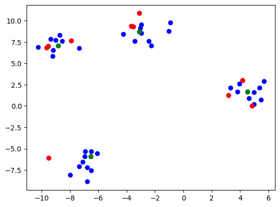
Then plotting the points and criticisms gets us

You’ll notice that I provided the option to use a separate kernel for prototype and criticism selection. This is because I’ve found that results for criticisms especially can be extremely sensitive to the sigma hyperparameter. This is an unfortunate limitation of the MMD Critic method and kernel methods in general. Overall, I’ve found good results using a large sigma for prototypes and a smaller one for criticisms.

We can also, of course, use a more complicated dataset. Here, for instance, is the method used on MNIST³:

from sklearn.datasets import fetch_openml
import numpy as np
from mmd_critic import MMDCritic
from mmd_critic.kernels import RBFKernel

# Load MNIST data
mnist = fetch_openml('mnist_784', version=1)
images = (mnist['data'].astype(np.float32)).to_numpy() / 255.0
labels = mnist['target'].astype(np.int64)


critic = MMDCritic(images[:15000], RBFKernel(2.5), RBFKernel(0.025))
protos, _ = critic.select_prototypes(40)
criticisms, _ = critic.select_criticisms(40, protos)

which gets us the following prototypes

and criticisms

Pretty neat, huh?

Conclusions

And that’s about it for the MMD-Critic method. It is quite simple at the core, and it is nice to use save for having to fiddle with the Sigma hyperparameter. I hope that the newly released Python package gives it more use.

Please contact [email protected] for any inquiries. All images by author unless stated otherwise.

Footnotes

[1] You may be familiar with RKHSs and kernels if you’ve ever studied SVMs and the kernel trick — the kernels used there are just inner products in some RKHS. The most common is the RBF kernel, for which the associated RKHS of functions is an infinite-dimensional set of smooth functions.

[2] I have not read this source beyond a brief skim. It seems mostly irrelevant, and the log determinant regularizer is fairly simple to implement. If you want to read it though, go for it.

[3] For legal reasons, you can find a repository with the MNIST dataset here. It is free for commercial use under the GPL-3.0 License.

References

[1] https://onlinelibrary.wiley.com/doi/book/10.1002/9780470316801
[2]https://proceedings.neurips.cc/paper_files/paper/2016/file/5680522b8e2bb01943234bce7bf84534-Paper.pdf
[3] https://f0nzie.github.io/interpretable_ml-rsuite/proto.html#examples-5
[4] https://jmlr.csail.mit.edu/papers/volume13/gretton12a/gretton12a.pdf
[5] https://www.stat.cmu.edu/~ryantibs/journalclub/mmd.pdf
[6] https://jmlr.org/papers/volume9/krause08a/krause08a.pdf

The MMD-Critic Method, Explained was originally published in Towards Data Science on Medium, where people are continuing the conversation by highlighting and responding to this story.