Blockchain analysts warn that the Russian government may use crypto exchanges like Garantex for sanctions evasion under the new legislation. The Russian government is likely to rely on domestic crypto exchanges like Garantex for sanctions evasion as it adapts to…
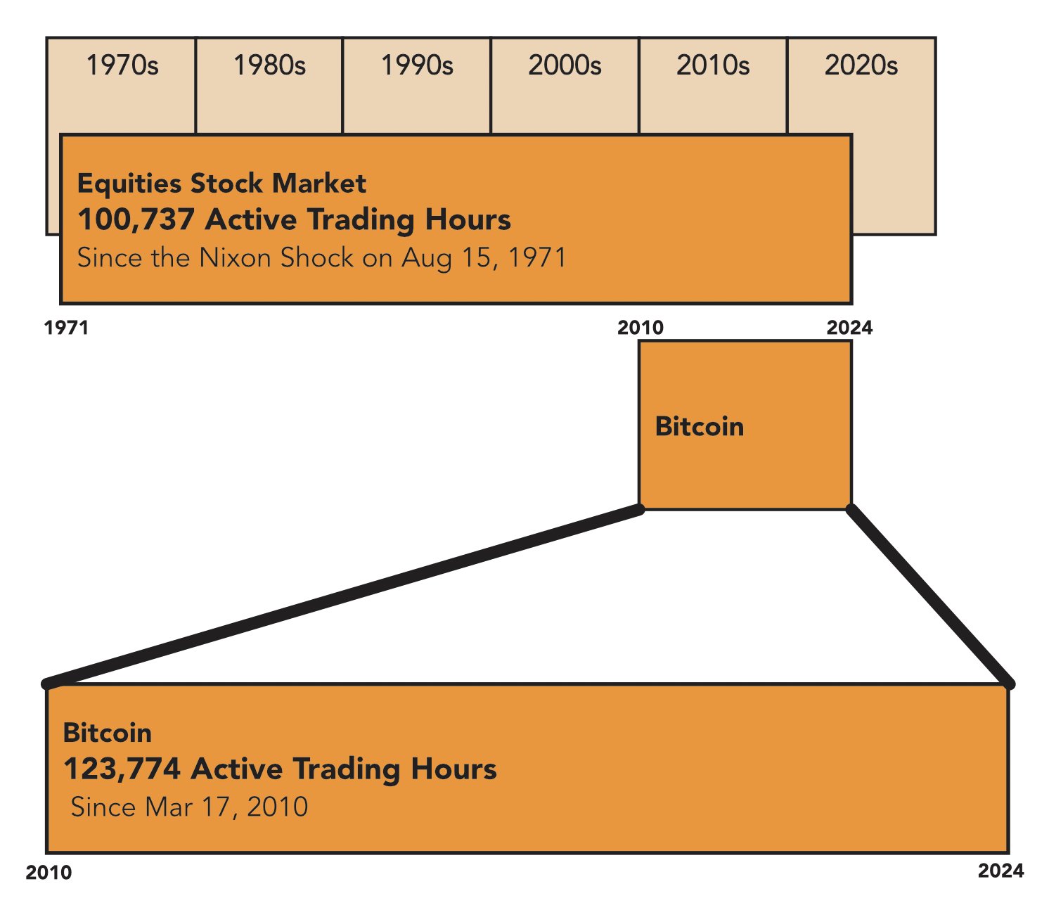
Bitcoin’s trading hours have surpassed those of the modern US fiat stock market since the Nixon Shock, but claims of it exceeding the entire history of US stock trading or fiat globally would be premature. A closer examination reveals a more nuanced picture of market longevity and trading activity. The crypto community recently buzzed with […]
Bitcoin’s mining sector is struggling, with revenue declining sharply
Transitioning to AI data centers might present significant cost and logistical challenges for Bitcoin miners
Experts believe that ETH might dip to the lower end of the falling wedge, currently around $2,200
Significant buying pressure can be seen around this zone too
Exploring popular reinforcement learning environments, in a beginner-friendly way
This is a guided series on introductory RL concepts using the environments from the OpenAI Gymnasium Python package. This first article will cover the high-level concepts necessary to understand and implement Q-learning to solve the “Frozen Lake” environment.
Happy learning ❤ !
A smiley lake (Image taken by author, made using OpenAI Gymnasium’s Frozen Lake environment)
Let’s explore reinforcement learning by comparing it to familiar examples from everyday life.
Card Game — Imagine playing a card game: When you first learn the game, the rules may be unclear. The cards you play might not be the most optimal and the strategies you use might be imperfect. As you play more and maybe win a few games, you learn what cards to play when and what strategies are better than others. Sometimes it’s better to bluff, but other times you should probably fold; saving a wild card for later use might be better than playing it immediately. Knowing what the optimal course of action is learned through a combination of experience and reward. Your experience comes from playing the game and you get rewarded when your strategies work well, perhaps leading to a victory or new high score.
A game of solitaire (Image taken by author from Google’s solitaire game)
Classical Conditioning — By ringing a bell before he fed a dog, Ivan Pavlov demonstrated the connection between external stimulus and a physiological response. The dog was conditioned to associate the sound of the bell with being fed and thus began to drool at the sound of the bell, even when no food was present. Though not strictly an example of reinforcement learning, through repeated experiences where the dog was rewarded with food at the sound of the bell, it still learned to associate the two together.
Feedback Control — An application of control theory found in engineering disciplines where a system’s behaviour can be adjusted by providing feedback to a controller. As a subset of feedback control, reinforcement learning requires feedback from our current environment to influence our actions. By providing feedback in the form of reward, we can incentivize our agent to pick the optimal course of action.
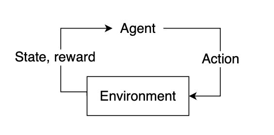
The Agent, State, and Environment
Reinforcement learning is a learning process built on the accumulation of past experiences coupled with quantifiable reward. In each example, we illustrate how our experiences can influence our actions and how reinforcing a positive association between reward and response could potentially be used to solve certain problems. If we can learn to associate reward with an optimal action, we could derive an algorithm that will select actions that yield the highest probable reward.
In reinforcement learning, the “learner” is called the agent. The agent interacts with our environment and, through its actions, learns what is considered “good” or “bad” based on the reward it receives.
The feedback cycle in reinforcement learning: Agent -> Action -> Environment -> Reward, State (Image by author)
To select a course of action, our agent needs some information about our environment, given by the state. The state represents current information about the environment, such as position, velocity, time, etc. Our agent does not necessarily know the entirety of the current state. The information available to our agent at any given point in time is referred to as an observation, which contains some subset of information present in the state. Not all states are fully observable, and some states may require the agent to proceed knowing only a small fraction of what might actually be happening in the environment. Using the observation, our agent must infer what the best possible action might be based on learned experience and attempt to select the action that yields the highest expected reward.
After selecting an action, the environment will then respond by providing feedback in the form of an updated state and reward. This reward will help us determine if the action the agent took was optimal or not.
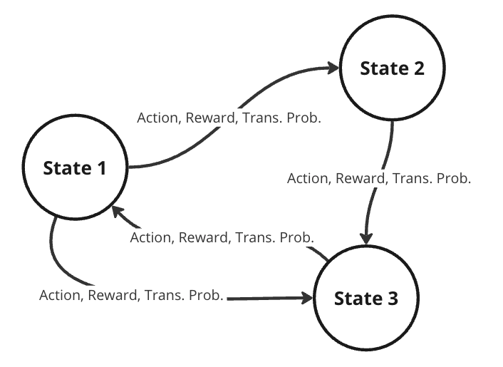
Markov Decision Processes (MDPs)
To better represent this problem, we might consider it as a Markov decision process (MDP). A MDP is a directed graph where each edge in the graph has a non-deterministic property. At each possible state in our graph, we have a set of actions we can choose from, with each action yielding some fixed reward and having some transitional probability of leading to some subsequent state. This means that the same actions are not guaranteed to lead to the same state every time since the transition from one state to another is not only dependent on the action, but the transitional probability as well.
Representation of a Markov decision process (Image by author)
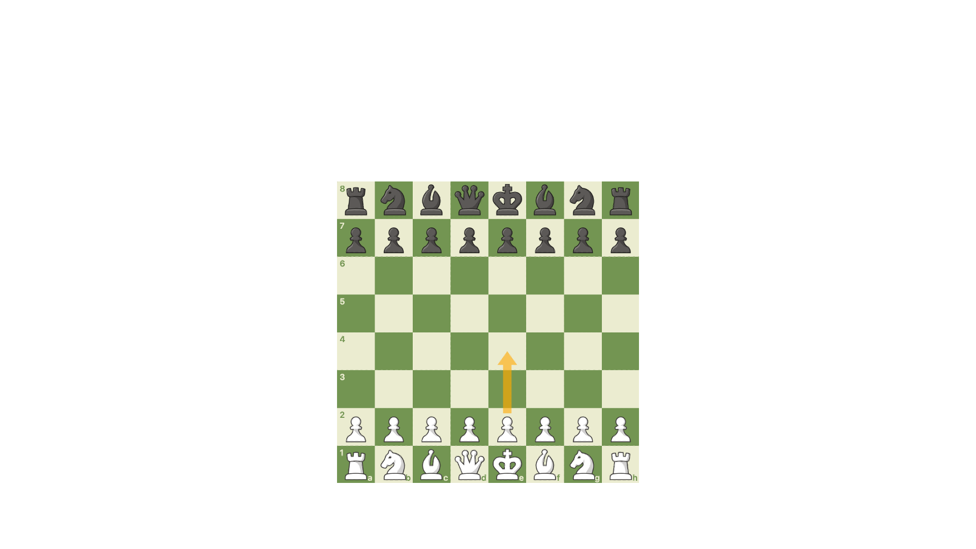
Randomness in decision models is useful in practical RL, allowing for dynamic environments where the agent lacks full control. Turn-based games like chess require the opponent to make a move before you can go again. If the opponent plays randomly, the future state of the board is never guaranteed, and our agent must play while accounting for a multitude of different probable future states. When the agent takes some action, the next state is dependent on what the opponent plays and is therefore defined by a probability distribution across possible moves for the opponent.
Animation showcasing that the state of the chess board is also dependent on what moves the opponent chooses to play (Image by author)
Our future state is therefore a function of both the probability of the agent selecting some action and the transitional probability of the opponent selecting some action. In general, we can assume that for any environment, the probability of our agent moving to some subsequent state from our current state is denoted by the joint probability of the agent selecting some action and the transitional probability of moving to that state.
Solving the MDP
To determine the optimal course of action, we want to provide our agent with lots of experience. Through repeated iterations of our environment, we aim to give the agent enough feedback that it can correctly choose the optimal action most, if not all, of the time. Recall our definition of reinforcement learning: a learning process built on the accumulation of past experiences coupled with quantifiable reward. After accumulating some experience, we want to use this experience to better select our future actions.
We can quantify our experiences by using them to predict the expected reward from future states. As we accumulate more experience, our predictions will become more accurate, converging to the true value after a certain number of iterations. For each reward that we receive, we can use that to update some information about our state, so the next time we encounter this state, we’ll have a better estimate of the reward that we might expect to receive.
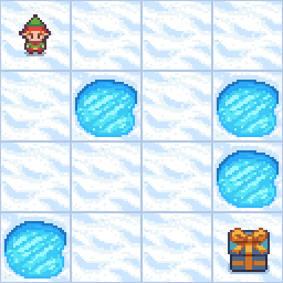
Frozen Lake Problem
Let’s consider consider a simple environment where our agent is a small character trying to navigate across a frozen lake, represented as a 2D grid. It can move in four directions: down, up, left, or right. Our goal is to teach it to move from its start position at the top left to an end position located at the bottom right of the map while avoiding the holes in the ice. If our agent manages to successfully reach its destination, we’ll give it a reward of +1. For all other cases, the agent will receive a reward of 0, with the added condition that if it falls into a hole, the exploration will immediately terminate.
Each state can be denoted by its coordinate position in the grid, with the start position in the top left denoted as the origin (0, 0), and the bottom right ending position denoted as (3, 3).
The most generic solution would be to apply some pathfinding algorithm to find the shortest path to from top left to bottom right while avoiding holes in the ice. However, the probability that the agent can move from one state to another is not deterministic. Each time the agent tries to move, there is a 66% chance that it will “slip” and move to a random adjacent state. In other words, there is only a 33% chance of the action the agent chose actually occurring. A traditional pathfinding algorithm cannot handle the introduction of a transitional probability. Therefore, we need an algorithm that can handle stochastic environments, aka reinforcement learning.
This problem can easily be represented as a MDP, with each state in our grid having some transitional probability of moving to any adjacent state. To solve our MDP, we need to find the optimal course of action from any given state. Recall that if we can find a way to accurately predict the future rewards from each state, we can greedily choose the best possible path by selecting whichever state yields the highest expected reward. We will refer to this predicted reward as the state-value. More formally, the state-value will define the expected reward gained starting from some state plus an estimate of the expected rewards from all future states thereafter, assuming we act according to the same policy of choosing the highest expected reward. Initially, our agent will have no knowledge of what rewards to expect, so this estimate can be arbitrarily set to 0.
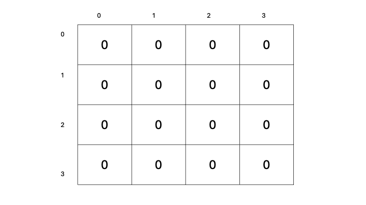
Let’s now define a way for us to select actions for our agent to take: We’ll begin with a table to store our predicted state-value estimates for each state, containing all zeros.
Table denoting the estimated state-value for each state in our grid (Image by author)
Our goal is to update these state-value estimates as we explore our environment. The more we traverse our environment, the more experience we will have, and the better our estimates will become. As our estimates improve, our state-values will become more accurate, and we will have a better representation of which states yield a higher reward, therefore allowing us to select actions based on which subsequent state has the highest state-value. This will surely work, right?
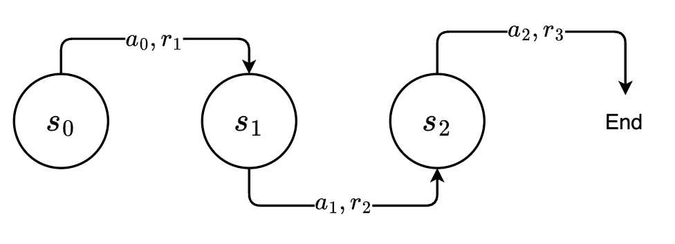
Visual representation of a single branch of our MDP (Image by author)
State-value vs. Action-value
Nope, sorry. One immediate problem that you might notice is that simply selecting the next state based on the highest possible state-value isn’t going to work. When we look at the set of possible next states, we aren’t considering our current action—that is, the action that we will take from our current state to get to the next one. Based on our definition of reinforcement learning, the agent-environment feedback loop always consists of the agent taking some action and the environment responding with both state and reward. If we only look at the state-values for possible next states, we are considering the reward that we would receive starting from those states, which completely ignores the action (and consequent reward) we took to get there. Additionally, trying to select a maximum across the next possible states assumes we can even make it there in the first place. Sometimes, being a little more conservative will help us be more consistent in reaching the end goal; however, this is out of the scope of this article :(.
Instead of evaluating across the set of possible next states, we’d like to directly evaluate our available actions. If our previous state-value function consisted of the expected rewards starting from the next state, we’d like to update this function to now include the reward from taking an action from the current state to get to the next state, plus the expected rewards from there on. We’ll call this new estimate that includes our current action action-value.
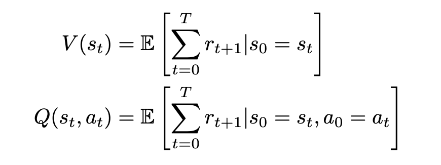
We can now formally define our state-value and action-value functions based on rewards and transitional probability. We’ll use expected value to represent the relationship between reward and transitional probability. We’ll denote our state-value as V and our action-value as Q, based on standard conventions in RL literature.
Equations for state- and action-value (Image by author)
The state-value V of some state s[t] is the expected sum of rewards r[t] at each state starting from s[t] to some future state s[T]; the action-value Q of some state s[t] is the expected sum of rewards r[t] at each state starting by taking an action a[t] to some future state-action pair s[T], a[T].
This definition is actually not the most accurate or conventional, and we’ll improve on it later. However, it serves as a general idea of what we’re looking for: a quantitative measure of future rewards.
Our state-value function V is an estimate of the maximum sum of rewards r we would obtain starting from state s and continually moving to the states that give the highest reward. Our action-value function is an estimate of the maximum reward we would obtain by taking action from some starting state and continually choosing the optimal actions that yield the highest reward thereafter. In both cases, we choose the optimal action/state to move to based on the expected reward that we would receive and loop this process until we either fall into a hole or reach our goal.
Greedy Policy & Return
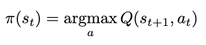
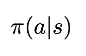
The method by which we choose our actions is called a policy. The policy is a function of state—given some state, it will output an action. In this case, since we want to select the next action based on maximizing the rewards, our policy can be defined as a function returning the action that yields the maximum action-value (Q-value) starting from our current state, or an argmax. Since we’re always selecting a maximum, we refer to this particular policy as greedy. We’ll denote our policy as a function of state s: π(s), formally defined as
Equation for the policy function = the action that yields the maximum estimated Q-value from some state s (Image by author)
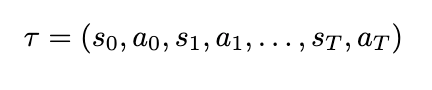
To simplify our notation, we can also define a substitution for our sum of rewards, which we’ll call return, and a substitution for a sequence of states and actions, which we’ll call a trajectory. A trajectory, denoted by the Greek letter τ (tau), is denoted as
Notation for trajectory: defined as some sequence of state-action pairs until some future timestep T. Defining the trajectory allows us to skip writing the entire sequence of states and actions, and substitute a single variable instead :P! (Image by author)
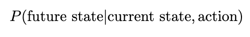
Since our environment is stochastic, it’s important to also consider the likelihood of such a trajectory occurring — low probability trajectories will reduce the expectation of reward. (Since our expected value consists of multiplying our reward by the transitional probability, trajectories that are less likely will have a lower expected reward compared to high probability ones.) The probability can be derived by considering the probability of each action and state happening incrementally: At any timestep in our MDP, we will select actions based on our policy, and the resulting state will be dependent on both the action we selected and the transitional probability. Without loss of generality, we’ll denote the transitional probability as a separate probability distribution, a function of both the current state and the attempted action. The conditional probability of some future state occurring is therefore defined as
Transitional probability of moving to a future state from a current state — for our frozen lake though, we know this value is fixed at ~0.33 (Image by author)
And the probability of some action happening based on our policy is simply evaluated by passing our state into our policy function
Expression for the probability of some action being selected by the policy given some state (Image by author)
Our policy is currently deterministic, as it selects actions based on the highest expected action-value. In other words, actions that have a low action-value will never be selected, while actions with a high Q-value will always be selected. This results in a Bernoulli distribution across possible actions. This is very rarely beneficial, as we’ll see later.
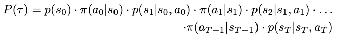
Applying these expressions to our trajectory, we can define the probability of some trajectory occurring as
Expanded equation for the probability of a certain trajectory occurring. Note that the probability of s0 is fixed at 1 assuming we start from the same state (top left) every time. (Image by author)
For clarity, here’s the original notation for a trajectory:
Notation for trajectory: defined as some sequence of state-action pairs until some future timestep T (Image by author)
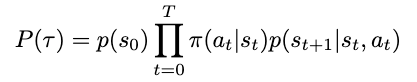
More concisely, we have
Concise notation for the probability of a trajectory occurring (Image by author)
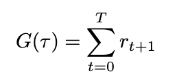
Defining both the trajectory and its probability allows us to substitute these expressions to simplify our definitions for both return and its expected value. The return (sum of rewards), which we’ll define as G based on conventions, can now be written as
Equation for return (Image by author)
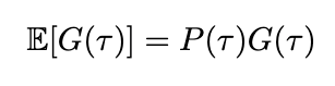
We can also define the expected return by introducing probability into the equation. Since we’ve already defined the probability of a trajectory, the expected return is therefore
Updated equation for expected return = the probability of the trajectory occurring times the return (Image by author)
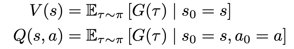
We can now adjust the definition of our value functions to include the expected return
Updated equations for state- and action-value (Image by author)
The main difference here is the addition of the subscript τ∼π indicating that our trajectory was sampled by following our policy (ie. our actions are selected based on the maximum Q-value). We’ve also removed the subscript t for clarity. Here’s the previous equation again for reference:
Equations for state- and action-value (Image by author)
Discounted Return
So now we have a fairly well-defined expression for estimating return but before we can start iterating through our environment, there’s still some more things to consider. In our frozen lake, it’s fairly unlikely that our agent will continue to explore indefinitely. At some point, it will slip and fall into a hole, and the episode will terminate. However, in practice, RL environments might not have clearly defined endpoints, and training sessions might go on indefinitely. In these situations, given an indefinite amount of time, the expected return would approach infinity, and evaluating the state- and action-value would become impossible. Even in our case, setting a hard limit for computing return is oftentimes not beneficial, and if we set the limit too high, we could end up with pretty absurdly large numbers anyway. In these situations, it is important to ensure that our reward series will converge using a discount factor. This improves stability in the training process and ensures that our return will always be a finite value regardless of how far into the future we look. This type of discounted return is also referred to as infinite horizon discounted return.
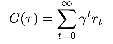
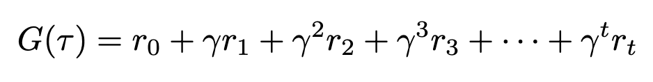
To add discounting to our return equation, we’ll introduce a new variable γ (gamma) to represent the discount factor.
Equation for discounted return (Image by author)
Gamma must always be less than 1, or our series will not converge. Expanding this expression makes this even more apparent
Expanded equation for discounted return (Image by author)
We can see that as time increases, gamma will be raised to a higher and higher power. As gamma is less than 1, raising it to a higher exponent will only make it smaller, thus exponentially decreasing the contribution of future rewards to the overall sum. We can substitute this updated definition of return back into our value functions, though nothing will visibly change since the variable is still the same.
Equations for state- and action-value, copied again for emphasis (Image by author)
Exploration vs. Exploitation
We mentioned earlier that always being greedy is not the best choice. Always selecting our actions based on the maximum Q-value will probably give us the highest chance of maximizing our reward, but that only holds when we have accurate estimates of those Q-values in the first place. To obtain accurate estimates, we need a lot of information, and we can only gain information by trying new things — that is, exploration.
When we select actions based on the highest estimated Q-value, we exploit our current knowledge base: we leverage our accumulated experiences in an attempt to maximize our reward. When we select actions based on any other metric, or even randomly, we explore alternative possibilities in an attempt to gain more useful information to update our Q-value estimates with. In reinforcement learning, we want to balance both exploration and exploitation. To properly exploit our knowledge, we need to have knowledge, and to gain knowledge, we need to explore.
Epsilon-Greedy Policy
We can balance exploration and exploitation by changing our policy from purely greedy to an epsilon-greedy one. An epsilon-greedy policy acts greedily most of the time with a probability of 1- ε, but has a probability of ε to act randomly. In other words, we’ll exploit our knowledge most of the time in an attempt to maximize reward, and we’ll explore occasionally to gain more knowledge. This is not the only way of balancing exploration and exploitation, but it is one of the simplest and easiest to implement.
Summary
Now the we’ve established a basis for understanding RL principles, we can move to discussing the actual algorithm — which will happen in the next article. For now, we’ll go over the high-level overview, combining all these concepts into a cohesive pseudo-code which we can delve into next time.
Q-Learning
The focus of this article was to establish the basis for understanding and implementing Q-learning. Q-learning consists of the following steps:
Initialize a tabular estimate of all action-values (Q-values), which we update as we iterate through our environment.
Select an action by sampling from our epsilon-greedy policy.
Collect the reward (if any) and update our estimate for our action-value.
Move to the next state, or terminate if we fall into a hole or reach the goal.
Loop steps 2–4 until our estimated Q-values converge.
Q-learning is an iterative process where we build estimates of action-value (and expected return), or “experience”, and use our experiences to identify which actions are the most rewarding for us to choose. These experiences are “learned” over many successive iterations of our environment and by leveraging them we will be able to consistently reach our goal, thus solving our MDP.
Glossary
Environment — anything that cannot be arbitrarily changed by our agent, aka the world around it
State — a particular condition of the environment
Observation — some subset of information from the state
Policy — a function that selects an action given a state
Agent — our “learner” which acts according to a policy in our environment
Reward — what our agent receives after performing certain actions
Return — a sum of rewards across a series of actions
Discounting — the process through which we ensure that our return does not reach infinity
State-value — the expected return starting from a state and continuing to act according to some policy, forever
Action-value — the expected return starting from a state and taking some action, and then continuing to act according to some policy, forever
Trajectory — a series of states and actions
Markov Decision Process (MDP) — the model we use to represent decision problems in RL aka a directed graph with non-deterministic edges
Exploration — how we obtain more knowledge
Exploitation — how we use our existing knowledge base to gain more reward
Q-Learning — a RL algorithm where we iteratively update Q-values to obtain better estimates of which actions will yield higher expected return
Reinforcement Learning — a learning process built on the accumulation of past experiences coupled with quantifiable reward
If you’ve read this far, consider leaving some feedback about the article — I’d appreciate it ❤.
References
[1] Gymnasium, Frozen Lake (n.d.), OpenAI Gymnasium Documentation.
Building real-world skills through hands-on trial and error.
The engaging discussions sparked by my recent blog post, “We Need to Raise the Bar for AI Product Managers,” highlighted a shared passion for advancing the field of AI product management. Many current and aspiring PMs have since reached out, asking how they can learn more about AI on their path to becoming an AI product manager.
In my experience, the most effective AI PMs excel in two key areas: identifying opportunities where AI can add value, and working with model developers to deploy the technology effectively. This requires a solid understanding of how different kinds of models are likely to behave when they go live — a reality that often surprises newcomers. The gap between flashy demos or early-stage prototypes and actual product performance can be substantial, whether you’re dealing with customer-facing applications or backend data pipelines that power products.
The best way to develop this intuition is by deploying a range of models into products and making plenty of mistakes along the way. The next best thing is to explore what other teams at your company are doing and learn from their mistakes (and triumphs). Dig up any documentation you can find and, where possible, listen in on product reviews or team updates. Often, people who worked directly on the projects will be happy to chat, answer your questions, and provide more context, especially if your team might be considering anything similar.
But what if you aren’t working at a company doing anything with AI? Or your company is focused on a very narrow set of technologies? Or maybe you’re in the midst of a job search?
In addition to checking out resources to familiarize yourself with terminology and best practices, I recommend developing your own AI projects. I actually recommend side projects even if you can learn a lot from your day job. Every AI use case has its own nuances, and the more examples you can get close to, the faster you’ll develop an intuition about what does and doesn’t work.
For a starter project, I recommend starting with LLMs like Claude or ChatGPT. You should be able to get something substantial up and running in a matter of hours (minutes if you already know how to code and write effective prompts). While not all AI projects at a real company will use LLMs, they are gaining significant traction. More importantly, it’s much easier to create your own working model with only rudimentary data science or coding knowledge. If your coding skills are rusty, using the developer APIs will give you a chance to brush up, and if you get stuck the LLM is a great resource to help with both code generation and troubleshooting. If you’re new to both coding and LLMs, then using the online chat interface is a great way to warm up.
Characteristics of a Good Starter Project
But what’s the difference between using the ChatGPT website or app to make you more productive (with requests like summarizing an article or drafting an email) versus an actual project?
A project should aim to solve a real problem in a repeatable way. It’s these nuances that will help you hone some of the most important skills for AI product management work at a company, especially model evaluation. Check out my article “What Exactly is an Eval and Why Should Product Managers Care” for an overview of model evaluation basics.
To ensure what you’re working on is a real project that can have its own mini eval, make sure you have:
Multiple test samples: Aim for projects where you can evaluate the model on at least 20 different examples or data points.
Diverse data: Ensure your dataset includes a variety of scenarios to test what causes the model to break (thus giving you more chances to fix it).
Clear evaluation criteria: Be clear from the start how an effective model or product behaves. You should have 20 ideal responses for your 20 examples to score the model.
Real-world relevance: Choose a problem that reflects actual use cases in your work, your personal life, or for someone close to you. You need to be well-informed to evaluate the model’s efficacy.
Sample Project Ideas
Please don’t do these specific projects unless one of them really speaks to you. These are for illustrative purposes only to help convey what makes a real project, versus a one-off query:
Gift Recommendation Classifier
Goal: Decide if a given product would be a good gift for an opinionated friend or family member.
Method: Use text generation to evaluate product titles and descriptions with a prompt describing the recipient’s taste profile. If you want to go a little more complex you could use vision capabilities to evaluate the product description and title AND a product image.
Test samples: 50 different product images and descriptions. To make this tricky, your examples should include some products that are obviously bad, some that obviously good, many that are borderline, and some that are completely random.
Evaluation: Have the target gift recipient evaluate the list of products, rating each on a scale (ex: “no way”, “meh” and “hell yes”) for how well it matches their preferences. Compare these ratings to the model’s classifications. You can also learn a lot from asking the model to give you a justification for why it thinks each item would or wouldn’t be a good match. This will help you troubleshoot failures and guide prompt updates, plus they will teach you a lot about how LLMs “think”.
Recipe Book Digitization
Goal: Convert your grandmother’s favorite out-of-print recipe book into an app for you and your cousins.
Method: Use vision capabilities to extract recipes from photos of the pages in a recipe book.
Test samples: 20 images of different types of recipes. To make it simpler to start, you could just focus on desserts. The examples might include 3 kinds of cookies, 4 kinds of cake, etc.
Evaluation: Are all the key ingredients and instructions from each included in the final output? Carefully compare the LLM output to the original recipe, checking for accuracy in ingredients, measurements, and cooking instructions. Bonus points if you can get the final data into some kind of structured format (e.g., JSON or CSV) for easier use in an app.
Image generated by the author using Midjourney
Public Figure Quote Extractor
Goal: Help a public figure’s publicity team identify any quote or fact said by them for your fact-checking team to verify.
Method: Use text generation to evaluate the text of articles and return a list of quotes and facts about your public figure mentioned in each article.
Test samples: 20 recent articles about the public figure covering at least 3 different events from at least 4 different publications (think one gossip site, one national paper like the New York Times, and something in between like Politico)
Evaluation: Read each article carefully and see if any facts or quotes from the public figure were missed. Imagine your job could be on the line if your summarizer hallucinates (ex: saying they said something they didn’t) or misses a key piece of misinformation. Check that all the quotes and facts the summarizer found are in fact related to your public figure, and also that they are all mentioned in the article.
You’re welcome to use any LLM for these projects, but in my experience, the ChatGPT API is the easiest to get started with if you have limited coding experience. Once you’ve successfully completed one project, evaluating another LLM on the same data is relatively straightforward.
Remember, the goal of starter projects isn’t perfection but to find an interesting project with some complexity to ensure you encounter difficulties. Learning to troubleshoot, iterate, and even hit walls where you realize something isn’t possible will help you hone your intuition for what is and isn’t feasible, and how much work is involved.
Embrace the learning process
Developing a strong intuition for AI capabilities and limitations is crucial for effective AI product management. By engaging in hands-on projects, you’ll gain invaluable experience in model evaluation, troubleshooting, and iteration. This practical knowledge will make you a more effective partner to model developers, enabling you to:
Identify areas where AI can truly add value
Make realistic estimates for AI project timelines and resourcing requirements
Contribute meaningfully to troubleshooting and evaluation processes
As you tackle these projects, you’ll develop a nuanced understanding of AI’s real-world applications and challenges. This experience will set you apart in the rapidly evolving field of AI product management, preparing you to lead innovative projects and make informed decisions that drive product success.
Remember, the journey to becoming an expert AI PM is ongoing. Embrace the learning process, stay curious, and continually seek out new challenges to refine your skills. With dedication and hands-on experience, you’ll be well-equipped to navigate the exciting frontier of AI product development.
Have questions about your AI project or this article? Connect with me on LinkedIn to continue the conversation.
Clustering is a must-have skill set for any data scientist due to its utility and flexibility to real-world problems. This article is an overview of clustering and the different types of clustering algorithms.
What is Clustering?
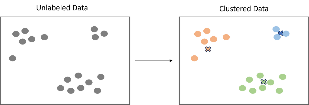
Clustering is a popular unsupervised learning technique that is designed to group objects or observations together based on their similarities. Clustering has a lot of useful applications such as market segmentation, recommendation systems, exploratory analysis, and more.
Image by Author
While clustering is a well-known and widely used technique in the field of data science, some may not be aware of the different types of clustering algorithms. While there are just a few, it is important to understand these algorithms and how they work to get the best results for your use case.
Centroid-Based Clustering
Centroid-based clustering is what most think of when it comes to clustering. It is the “traditional” way to cluster data by using a defined number of centroids (centers) to group data points based on their distance to each centroid. The centroid ultimately becomes the mean of it’s assigned data points. While centroid-based clustering is powerful, it is not robust against outliers, as outliers will need to be assigned to a cluster.
K-Means
K-Means is the most widely used clustering algorithm, and is likely the first one you will learn as a data scientist. As explained above, the objective is to minimize the sum of distances between the data points and the cluster centroid to identify the correct group that each data point should belong to. Here’s how it works:
A defined number of centroids are randomly dropped into the vector space of the unlabeled data (initialization).
Each data point measures itself to each centroid (usually using Euclidean distance) and assigns itself to the closest one.
The centroids relocate to the mean of their assigned data points.
Steps 2–3 repeat until the ‘optimal’ clusters are produced.
Image by Author
from sklearn.cluster import KMeans import numpy as np
#sample data X = np.array([[1, 2], [1, 4], [1, 0], [10, 2], [10, 4], [10, 0]])
#print the results, use to predict, and print centers kmeans.labels_ kmeans.predict([[0, 0], [12, 3]]) kmeans.cluster_centers_
K-Means ++
K-Means ++ is an improvement of the initialization step of K-Means. Since the centroids are randomly dropped in, there is a chance that more than one centroid might be initialized into the same cluster, resulting in poor results.
However K-Means ++ solves this by randomly assigning the first centroid that will eventually find the largest cluster. Then, the other centroids are placed a certain distance away from the initial cluster. The goal of K-Means ++ is to push the centroids as far as possible from one another. This results in high-quality clusters that are distinct and well-defined.
from sklearn.cluster import KMeans import numpy as np
#sample data X = np.array([[1, 2], [1, 4], [1, 0], [10, 2], [10, 4], [10, 0]])
#print the results, use to predict, and print centers kmeans.labels_ kmeans.predict([[0, 0], [12, 3]]) kmeans.cluster_centers_
Density-Based Clustering
Density-based algorithms are also a popular form of clustering. However, instead of measuring from randomly placed centroids, they create clusters by identifying high-density areas within the data. Density-based algorithms do not require a defined number of clusters, and therefore are less work to optimize.
While centroid-based algorithms perform better with spherical clusters, density-based algorithms can take arbitrary shapes and are more flexible. They also do not include outliers in their clusters and therefore are robust. However, they can struggle with data of varying densities and high dimensions.
Image by Author
DBSCAN
DBSCAN is the most popular density-based algorithm. DBSCAN works as follows:
DBSCAN randomly selects a data point and checks if it has enough neighbors within a specified radius.
If the point has enough neighbors, it is marked as part of a cluster.
DBSCAN recursively checks if the neighbors also have enough neighbors within the radius until all points in the cluster have been visited.
Repeat steps 1–3 until the remaining data point do not have enough neighbors in the radius.
Remaining data points are marked as outliers.
from sklearn.cluster import DBSCAN
import numpy as np

#sample data
X = np.array([[1, 2], [2, 2], [2, 3],
              [8, 7], [8, 8], [25, 80]])

#create model
clustering = DBSCAN(eps=3, min_samples=2).fit(X)

#print results
clustering.labels_
Hierarchical Clustering
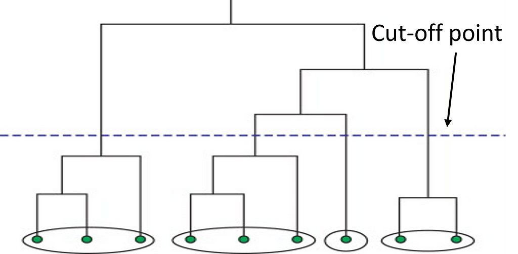
Next, we have hierarchical clustering. This method starts off by computing a distance matrix from the raw data. This distance matrix is best and often visualized by a dendrogram (see below). Data points are linked together one by one by finding the nearest neighbor to eventually form one giant cluster. Therefore, a cut-off point to identify the clusters by stopping all data points from linking together.
Image by Author
By using this method, the data scientist can build a robust model by defining outliers and excluding them in the other clusters. This method works great against hierarchical data, such as taxonomies. The number of clusters depends on the depth parameter and can be anywhere from 1-n.
from scipy.cluster.hierarchy import dendrogram, linkage from sklearn.cluster import AgglomerativeClustering from scipy.cluster.hierarchy import fcluster
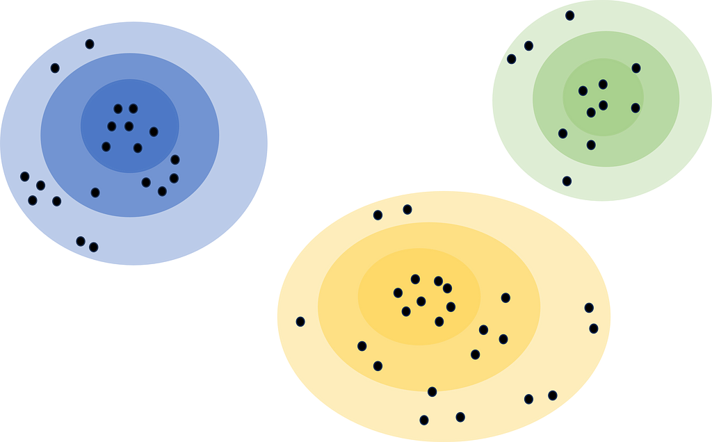
Lastly, distribution-based clustering considers a metric other than distance and density, and that is probability. Distribution-based clustering assumes that the data is made up of probabilistic distributions, such as normal distributions. The algorithm creates ‘bands’ that represent confidence intervals. The further away a data point is from the center of a cluster, the less confident we are that the data point belongs to that cluster.
Image by Author
Distribution-based clustering is very difficult to implement due to the assumptions it makes. It usually is not recommended unless rigorous analysis has been done to confirm its results. For example, using it to identify customer segments in a marketing dataset, and confirming these segments follow a distribution. This can also be a great method for exploratory analysis to see not only what the centers of clusters comprise of, but also the edges and outliers.
Conclusion
Clustering is an unsupervised machine learning technique that has a growing utility in many fields. It can be used to support data analysis, segmentation projects, recommendation systems, and more. Above we have explored how they work, their pros and cons, code samples, and even some use cases. I would consider experience with clustering algorithms a must-have for data scientists due to their utility and flexibility.
I hope you have enjoyed my article! Please feel free to comment, ask questions, or request other topics.
We use cookies on our website to give you the most relevant experience by remembering your preferences and repeat visits. By clicking “Accept”, you consent to the use of ALL the cookies.
This website uses cookies to improve your experience while you navigate through the website. Out of these, the cookies that are categorized as necessary are stored on your browser as they are essential for the working of basic functionalities of the website. We also use third-party cookies that help us analyze and understand how you use this website. These cookies will be stored in your browser only with your consent. You also have the option to opt-out of these cookies. But opting out of some of these cookies may affect your browsing experience.
Necessary cookies are absolutely essential for the website to function properly. These cookies ensure basic functionalities and security features of the website, anonymously.
Cookie
Duration
Description
cookielawinfo-checkbox-analytics
11 months
This cookie is set by GDPR Cookie Consent plugin. The cookie is used to store the user consent for the cookies in the category "Analytics".
cookielawinfo-checkbox-functional
11 months
The cookie is set by GDPR cookie consent to record the user consent for the cookies in the category "Functional".
cookielawinfo-checkbox-necessary
11 months
This cookie is set by GDPR Cookie Consent plugin. The cookies is used to store the user consent for the cookies in the category "Necessary".
cookielawinfo-checkbox-others
11 months
This cookie is set by GDPR Cookie Consent plugin. The cookie is used to store the user consent for the cookies in the category "Other.
cookielawinfo-checkbox-performance
11 months
This cookie is set by GDPR Cookie Consent plugin. The cookie is used to store the user consent for the cookies in the category "Performance".
viewed_cookie_policy
11 months
The cookie is set by the GDPR Cookie Consent plugin and is used to store whether or not user has consented to the use of cookies. It does not store any personal data.
Functional cookies help to perform certain functionalities like sharing the content of the website on social media platforms, collect feedbacks, and other third-party features.
Performance cookies are used to understand and analyze the key performance indexes of the website which helps in delivering a better user experience for the visitors.
Analytical cookies are used to understand how visitors interact with the website. These cookies help provide information on metrics the number of visitors, bounce rate, traffic source, etc.
Advertisement cookies are used to provide visitors with relevant ads and marketing campaigns. These cookies track visitors across websites and collect information to provide customized ads.