Blog

A gentle introduction to mechanistic interpretability through simple algorithmic examples

Introduction

This article shows how small Artificial Neural Networks (NN) can represent basic functions. The goal is to provide fundamental intuition about how NNs work and to serve as a gentle introduction to Mechanistic Interpretability — a field that seeks to reverse engineer NNs.

I present three examples of elementary functions, describe each using a simple algorithm, and show how the algorithm can be “coded” into the weights of a neural network. Then, I explore if the network can learn the algorithm using backpropagation. I encourage readers to think about each example as a riddle and take a minute before reading the solution.

Machine Learning Topology

This article attempts to break NNs into discrete operations and describe them as algorithms. An alternative approach, perhaps more common and natural, is looking at the continuous topological interpretations of the linear transformations in different layers.

The following are some great resources for strengthening your topological intuition:

• Tensorflow Playground — a simple tool for building basic intuition on classification tasks.
• ConvnetJS Demo — a more sophisticated tool for visualizing NNs for classification tasks.
• Neural Networks, Manifolds, and Topology — a great article for building topological intuition of how NNs work.

Three Elementary Functions

In all the following examples, I use the terminology “neuron” for a single node in the NN computation graph. Each neuron can be used only once (no cycles; e.g., not RNN), and it performs 3 operations in the following order:

1. Inner product with the input vector.
2. Adding a bias term.
3. Running a (non-linear) activation function.

I provide only minimal code snippets so that reading will be fluent. This Colab notebook includes the entire code.

The < operator

How many neurons are required to learn the function “x < 10”? Write an NN that returns 1 when the input is smaller than 10 and 0 otherwise.

Solution

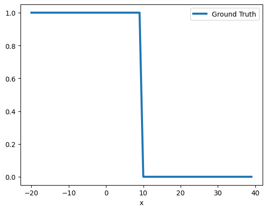
Let’s start by creating sample dataset that follows the pattern we want to learn

X = [[i] for i in range(-20, 40)]
Y = [1 if z[0] < 10 else 0 for z in X]

This classification task can be solved using logistic regression and a Sigmoid as the output activation. Using a single neuron, we can write the function as Sigmoid(ax+b). b, the bias term, can be thought of as the neuron’s threshold. Intuitively, we can set b = 10 and a = -1 and get F=Sigmoid(10-x)

Let’s implement and run F using PyTorch

model = nn.Sequential(nn.Linear(1,1), nn.Sigmoid())
d = model.state_dict()
d["0.weight"] = torch.tensor([[-1]]).float()
d['0.bias'] = torch.tensor([10]).float()
model.load_state_dict(d)
y_pred = model(x).detach().reshape(-1)

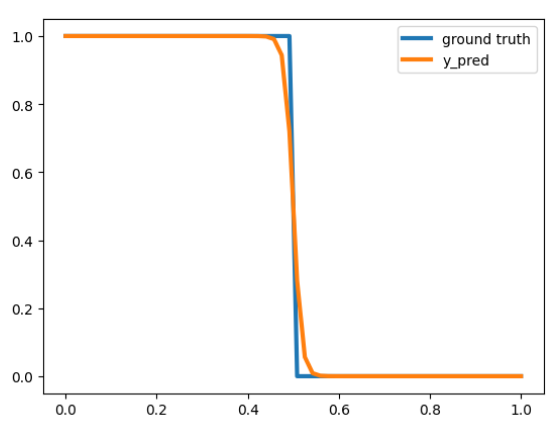
Seems like the right pattern, but can we make a tighter approximation? For example, F(9.5) = 0.62, we prefer it to be closer to 1.

For the Sigmoid function, as the input approaches -∞ / ∞ the output approaches 0 / 1 respectively. Therefore, we need to make our 10 — x function return large numbers, which can be done by multiplying it by a larger number, say 100, to get F=Sigmoid(100(10-x)), now we’ll get F(9.5) =~1.

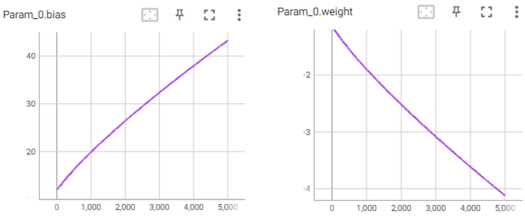
Indeed, when training a network with one neuron, it converges to F=Sigmoid(M(10-x)), where M is a scalar that keeps growing during training to make the approximation tighter.

To clarify, our single-neuron model is only an approximation of the “<10” function. We will never be able to reach a loss of zero, because the neuron is a continuous function while “<10” is not a continuous function.

Min(a, b)

Write a neural network that takes two numbers and returns the minimum between them.

Solution

Like before, let’s start by creating a test dataset and visualizing it

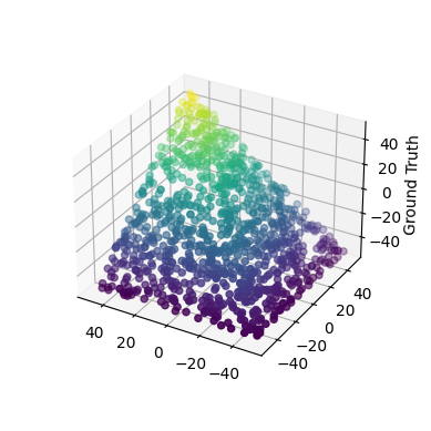
X_2D = [
[random.randrange(-50, 50),
 random.randrange(-50, 50)]
 for i in range(1000)
]
Y = [min(a, b) for a, b in X_2D]

In this case, ReLU activation is a good candidate because it is essentially a maximum function (ReLU(x) = max(0, x)). Indeed, using ReLU one can write the min function as follows

min(a, b) = 0.5 (a + b -|a - b|) = 0.5 (a + b - ReLU(b - a) - ReLU(a - b))

[Equation 1]

Now let’s build a small network that is capable of learning Equation 1, and try to train it using gradient descent

class MinModel(nn.Module):
  def __init__(self):
      super(MinModel, self).__init__()

      # For ReLU(a-b)
      self.fc1 = nn.Linear(2, 1)
      self.relu1 = nn.ReLU()
      # For ReLU(b-a)
      self.fc2 = nn.Linear(2, 1)
      self.relu2 = nn.ReLU()
      # Takes 4 inputs
      # [a, b, ReLU(a-b), ReLU(b-a)]
      self.output_layer = nn.Linear(4, 1)

  def forward(self, x):
      relu_output1 = self.relu1(self.fc1(x))
      relu_output2 = self.relu2(self.fc2(x))
      return self.output_layer(
          torch.cat(
             (x, Relu_output1, relu_output2),
             dim=-1
          )
      )

Training for 300 epochs is enough to converge. Let’s look at the model’s parameters

>> for k, v in model.state_dict().items():
>>   print(k, ": ", torch.round(v, decimals=2).numpy())

fc1.weight :  [[-0. -0.]]
fc1.bias :  [0.]
fc2.weight :  [[ 0.71 -0.71]]
fc2.bias :  [-0.]
output_layer.weight :  [[ 1.    0.    0.   -1.41]]
output_layer.bias :  [0.]

Many weights are zeroing out, and we are left with the nicely looking

model([a,b]) = a - 1.41 * 0.71 ReLU(a-b) ≈ a - ReLU(a-b)

This is not the solution we expected, but it is a valid solution and even cleaner than Equation 1! By looking at the network we learned a new nicely looking formula! Proof:

Proof:

• If a <= b: model([a,b]) = a — ReLU(a-b) = a — 0 = a
• If a > b: a — ReLU(a-b) = a — (a-b) = b

Is even?

Create a neural network that takes an integer x as an input and returns x mod 2. That is, 0 if x is even, 1 if x is odd.

This one looks quite simple, but surprisingly it is impossible to create a finite-size network that correctly classifies each integer in (-∞, ∞) (using a standard non-periodic activation function such as ReLU).

Theorem: is_even needs at least log neurons

A network with ReLU activations requires at least n neurons to correctly classify each of 2^n consecutive natural numbers as even or odd (i.e., solving is_even).

Proof: Using Induction

Base: n == 2: Intuitively, a single neuron (of the form ReLU(ax + b)), cannot solve S = [i + 1, i + 2, i + 3, i + 4] as it is not linearly separable. For example, without loss of generality, assume a > 0 and i + 2 is even. If ReLU(a(i + 2) + b) = 0, then also ReLU(a(i + 1) + b) = 0 (monotonic function), but i + 1 is odd.
More details are included in the classic Perceptrons book.

Assume for n, and look at n+1: Let S = [i + 1, …, i + 2^(n + 1)], and assume, for the sake of contradiction, that S can be solved using a network of size n. Take an input neuron from the first layer f(x) = ReLU(ax + b), where x is the input to the network. WLOG a > 0. Based on the definition of ReLU there exists a j such that:
S’ = [i + 1, …, i + j], S’’ = [i + j + 1, …, i + 2^(n + 1)]
f(x ≤ i) = 0
f(x ≥ i) = ax + b

There are two cases to consider:

• Case |S’| ≥ 2^n: dropping f and all its edges won’t change the classification results of the network on S’. Hence, there is a network of size n-1 that solves S’. Contradiction.
• Case |S’’|≥ 2^n: For each neuron g which takes f as an input g(x) = ReLU(cf(x) + d + …) = ReLU(c ReLU(ax + b) + d + …), Drop the neuron f and wire x directly to g, to get ReLU(cax + cb + d + …). A network of size n — 1 solves S’’. Contradiction.

Logarithmic Algorithm

How many neurons are sufficient to classify [1, 2^n]? I have proven that n neurons are necessary. Next, I will show that n neurons are also sufficient.

One simple implementation is a network that constantly adds/subtracts 2, and checks if at some point it reaches 0. This will require O(2^n) neurons. A more efficient algorithm is to add/subtract powers of 2, which will require only O(n) neurons. More formally:
f_i(x) := |x — i|
f(x) := f_1∘ f_1∘ f_2 ∘ f_4∘ … ∘ f_(2^(n-1)) (|x|)

Proof:

• By definition:∀ x ϵ[0, 2^i]: f_(2^(i-1)) (x) ≤ 2^(i-1).
  I.e., cuts the interval by half.
• Recursively f_1∘ f_1∘ f_2 ∘ … ∘ f_(2^(n-1)) (|x|) ≤ 1
• For every even i: is_even(f_i(x)) = is_even(x)
• Similarly is_even(f_1( f_1(x))) = is_even(x)
• We got f(x) ϵ {0,1} and is_even(x) =is_even(f(x)). QED.

Implementation

Let’s try to implement this algorithm using a neural network over a small domain. We start again by defining the data.

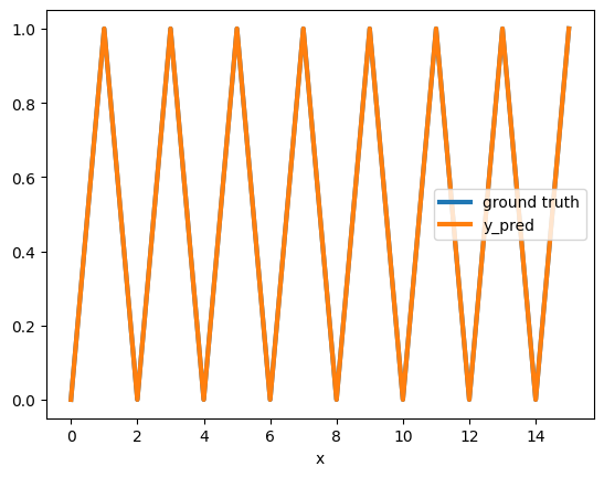
X = [[i] for i in range(0, 16)]
Y = [z[0] % 2 for z in X]

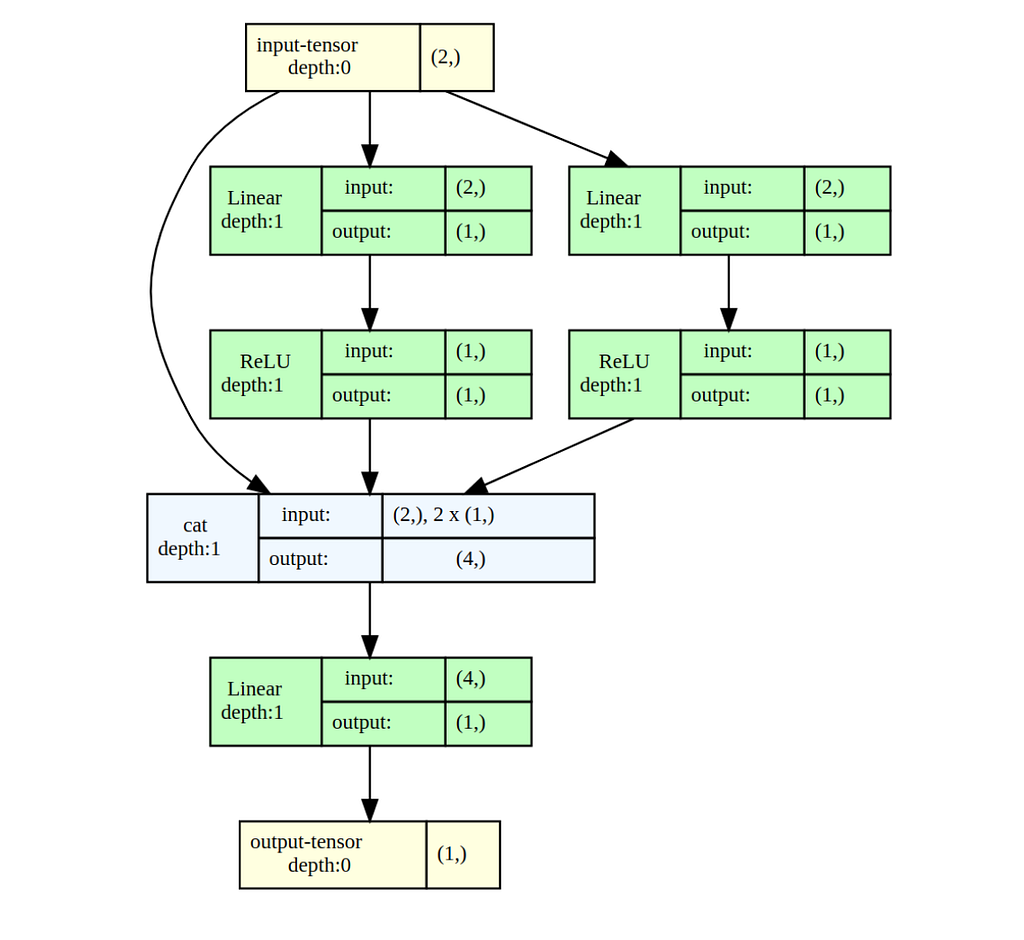
Because the domain contains 2⁴ integers, we need to use 6 neurons. 5 for f_1∘ f_1∘ f_2 ∘ f_4∘ f_8, + 1 output neuron. Let’s build the network and hardwire the weights

def create_sequential_model(layers_list = [1,2,2,2,2,2,1]):
  layers = []
  for i in range(1, len(layers_list)):
      layers.append(nn.Linear(layers_list[i-1], layers_list[i]))
      layers.append(nn.ReLU())
  return nn.Sequential(*layers)

# This weight matrix implements |ABS| using ReLU neurons.
# |x-b| = Relu(-(x-b)) + Relu(x-b)
abs_weight_matrix = torch_tensor([[-1, -1],
                                  [1, 1]])
# Returns the pair of biases used for each of the ReLUs.
get_relu_bias = lambda b: torch_tensor([b, -b])

d = model.state_dict()
d['0.weight'], d['0.bias'] = torch_tensor([[-1],[1]]), get_relu_bias(8)
d['2.weight'], d['2.bias'] = abs_weight_matrix, get_relu_bias(4)
d['4.weight'], d['4.bias'] = abs_weight_matrix, get_relu_bias(2)
d['6.weight'], d['6.bias'] = abs_weight_matrix, get_relu_bias(1)
d['8.weight'], d['8.bias'] = abs_weight_matrix, get_relu_bias(1)
d['10.weight'], d['10.bias'] = torch_tensor([[1, 1]]), torch_tensor([0])
model.load_state_dict(d)
model.state_dict()

As expected we can see that this model makes a perfect prediction on [0,15]

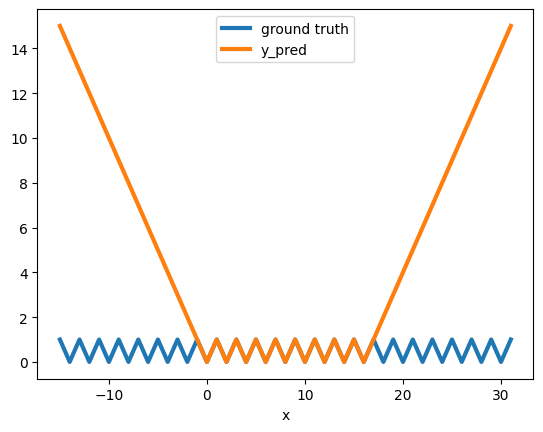
And, as expected, it doesn’t generalizes to new data points

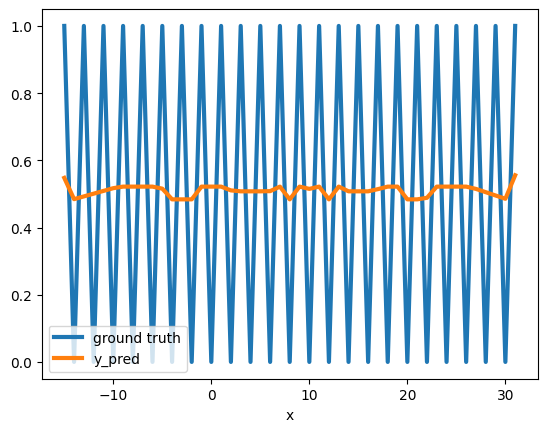
We saw that we can hardwire the model, but would the model converge to the same solution using gradient descent?

The answer is — not so easily! Instead, it is stuck at a local minimum — predicting the mean.

This is a known phenomenon, where gradient descent can get stuck at a local minimum. It is especially prevalent for non-smooth error surfaces of highly nonlinear functions (such as is_even).

More details are beyond the scope of this article, but to get more intuition one can look at the many works that investigated the classic XOR problem. Even for such a simple problem, we can see that gradient descent can struggle to find a solution. In particular, I recommend Richard Bland’s short book “Learning XOR: exploring the space of a classic problem” — a rigorous analysis of the error surface of the XOR problem.

Final Words

I hope this article has helped you understand the basic structure of small neural networks. Analyzing Large Language Models is much more complex, but it’s an area of research that is advancing rapidly and is full of intriguing challenges.

When working with Large Language Models, it’s easy to focus on supplying data and computing power to achieve impressive results without understanding how they operate. However, interpretability offers crucial insights that can help address issues like fairness, inclusivity, and accuracy, which are becoming increasingly vital as we rely more on LLMs in decision-making.

For further exploration, I recommend following the AI Alignment Forum.

*All the images were created by the author. The intro image was created using ChatGPT and the rest were created using Python libraries.

---

How Tiny Neural Networks Represent Basic Functions was originally published in Towards Data Science on Medium, where people are continuing the conversation by highlighting and responding to this story.