Blog

Exploring the foundations, concepts, and math of kernel density estimation

The Kernel Density Estimator is a fundamental non-parametric method that is a versatile tool for uncovering the hidden distributions of your data. This article delves into the mathematical foundations of the estimator, provides guidance on choosing the optimal bandwidth, and briefly touches on the choice of kernel functions and other related topics.

Part 1: Introduction

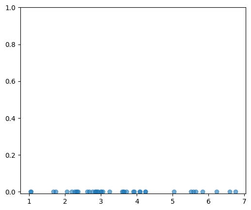
Suppose I give you the following sample of data:

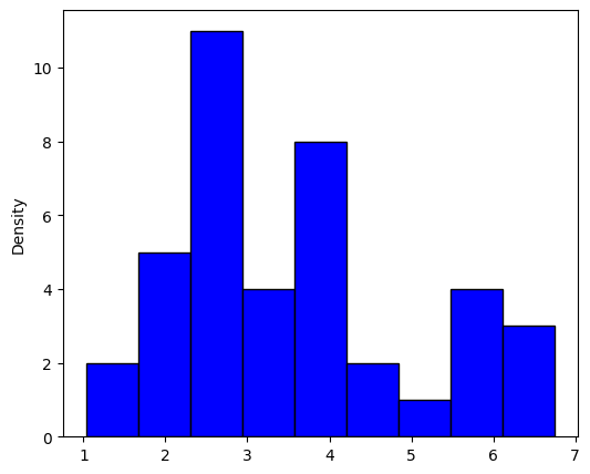
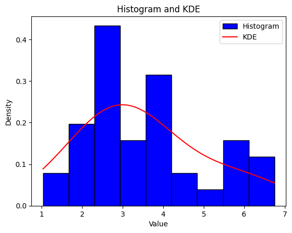
One of the first and easiest steps in analyzing sample data is to generate a histogram, for our data we get the following:

Not very useful, and we are no closer to understanding what the underlying distribution is. There is also the additional problem that, in practice, data rarely exhibit the sharp rectangular structure produced by a histogram. The kernel density estimator provides a remedy, and it is a non-parametric way to estimate the probability density function of a random variable.

import numpy as np
import matplotlib.pyplot as plt
from sklearn.neighbors import KernelDensity

# Generate sample data
np.random.seed(14)
uniform_data = np.random.uniform(low=1, high=7, size=20)
normal_data = np.random.normal(loc=3, scale=0.7, size=20)

# Combine both distributions
combined_data = np.concatenate([uniform_data, normal_data])

# Compute histogram
hist, bin_edges = np.histogram(combined_data, bins=9, density=True)

# Compute KDE
kde = KernelDensity(kernel='gaussian').fit(combined_data[:, None])
x = np.linspace(min(combined_data), max(combined_data), 1000)[:, None]
log_density = kde.score_samples(x)
density = np.exp(log_density)

# Plot histogram
plt.hist(combined_data, bins=9, density=True, color='blue', edgecolor='black', label='Histogram')

# Plot KDE
plt.plot(x, density, color='red', label='KDE')

# Add labels and legend
plt.ylabel('Density')
plt.title('Histogram and KDE')
plt.legend()

# Show plot
plt.show()

Part 2: Derivation

The following derivation takes inspiration from Bruce E. Hansen’s “Lecture Notes on Nonparametric” (2009). If you are interested in learning more you can refer to his original lecture notes here.

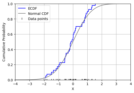
Suppose we wanted to estimate a probability density function, f(t), from a sample of data. A good starting place would be to estimate the cumulative distribution function, F(t), using the empirical distribution function (EDF). Let X1, …, Xn be independent, identically distributed real random variables with the common cumulative distribution function F(t). The EDF is defined as:

Then, by the strong law of large numbers, as n approaches infinity, the EDF converges almost surely to F(t). Now, the EDF is a step function that could look like the following:

import numpy as np
import matplotlib.pyplot as plt
from scipy.stats import norm

# Generate sample data
np.random.seed(14)
data = np.random.normal(loc=0, scale=1, size=40)

# Sort the data
data_sorted = np.sort(data)

# Compute ECDF values
ecdf_y = np.arange(1, len(data_sorted)+1) / len(data_sorted)

# Generate x values for the normal CDF
x = np.linspace(-4, 4, 1000)
cdf_y = norm.cdf(x)

# Create the plot
plt.figure(figsize=(6, 4))
plt.step(data_sorted, ecdf_y, where='post', color='blue', label='ECDF')
plt.plot(x, cdf_y, color='gray', label='Normal CDF')
plt.plot(data_sorted, np.zeros_like(data_sorted), '|', color='black', label='Data points')

# Label axes
plt.xlabel('X')
plt.ylabel('Cumulative Probability')

# Add grid
plt.grid(True)

# Set limits
plt.xlim([-4, 4])
plt.ylim([0, 1])

# Add legend
plt.legend()

# Show plot
plt.show()

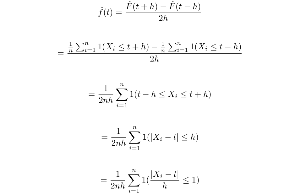
Therefore, if we were to try and find an estimator for f(t) by taking the derivative of the EDF, we would get a scaled sum of Dirac delta functions, which is not very helpful. Instead let us consider using the two-point central difference formula of the estimator as an approximation of the derivative. Which, for a small h>0, we get:

Now define the function k(u) as follows:

Then we have that:

Which is a special case of the kernel density estimator, where here k is the uniform kernel function. More generally, a kernel function is a non-negative function from the reals to the reals which satisfies:

We will assume that all kernels discussed in this article are symmetric, hence we have that k(-u) = k(u).

The moment of a kernel, which gives insights into the shape and behavior of the kernel function, is defined as the following:

Lastly, the order of a kernel is defined as the first non-zero moment.

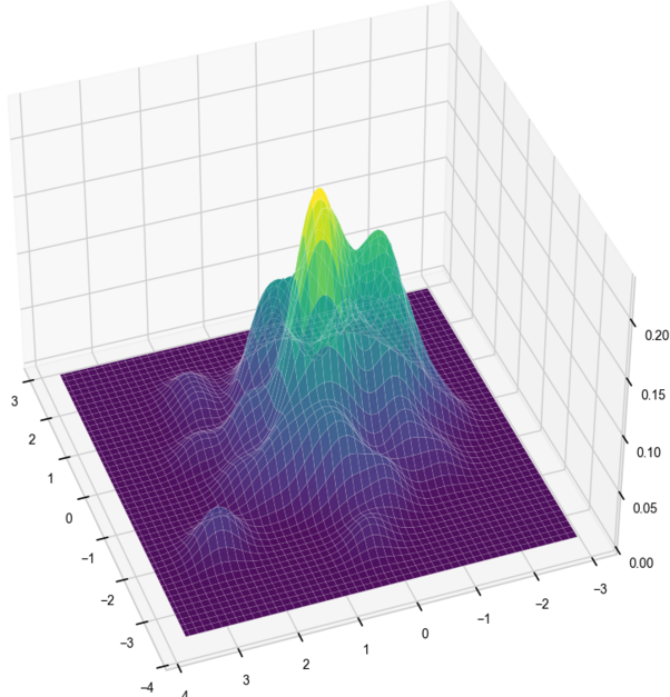
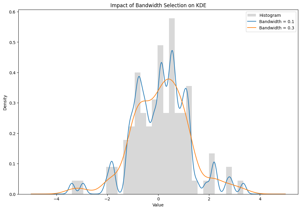
We can only minimize the error of the kernel density estimator by either changing the h value (bandwidth), or the kernel function. The bandwidth parameter has a much larger impact on the resulting estimate than the kernel function but is also much more difficult to choose. To demonstrate the influence of the h value, take the following two kernel density estimates. A Gaussian kernel was used to estimate a sample generated from a standard normal distribution, the only difference between the estimators is the chosen h value.

import numpy as np
import matplotlib.pyplot as plt
from scipy.stats import gaussian_kde

# Generate sample data
np.random.seed(14)
data = np.random.normal(loc=0, scale=1, size=100)

# Define the bandwidths
bandwidths = [0.1, 0.3]

# Plot the histogram and KDE for each bandwidth
plt.figure(figsize=(12, 8))
plt.hist(data, bins=30, density=True, color='gray', alpha=0.3, label='Histogram')

x = np.linspace(-5, 5, 1000)
for bw in bandwidths:
    kde = gaussian_kde(data , bw_method=bw)
    plt.plot(x, kde(x), label=f'Bandwidth = {bw}')

# Add labels and title
plt.title('Impact of Bandwidth Selection on KDE')
plt.xlabel('Value')
plt.ylabel('Density')
plt.legend()
plt.show()

Quite a dramatic difference.

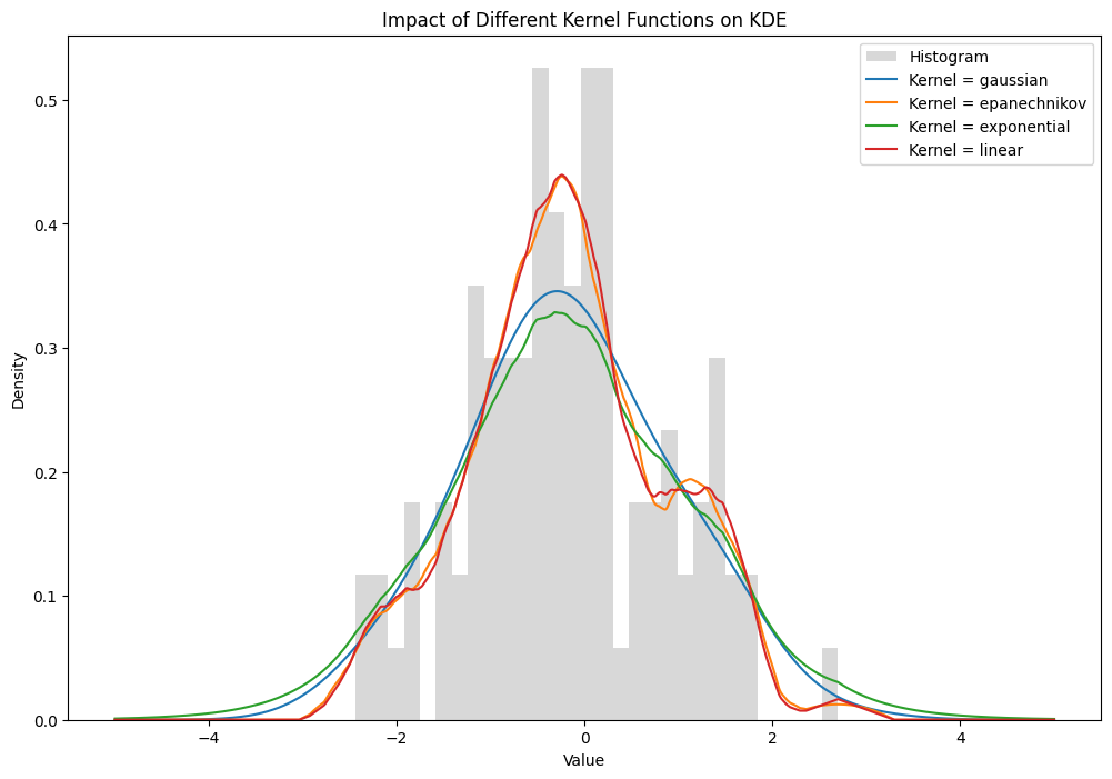
Now let us look at the impact of changing the kernel function while keeping the bandwidth constant.

import numpy as np
import matplotlib.pyplot as plt
from sklearn.neighbors import KernelDensity

# Generate sample data
np.random.seed(14)
data = np.random.normal(loc=0, scale=1, size=100)[:, np.newaxis]  # reshape for sklearn

# Intialize a constant bandwidth
bandwidth = 0.6

# Define different kernel functions
kernels = ["gaussian", "epanechnikov", "exponential", "linear"]

# Plot the histogram (transparent) and KDE for each kernel
plt.figure(figsize=(12, 8))

# Plot the histogram
plt.hist(data, bins=30, density=True, color="gray", alpha=0.3, label="Histogram")

# Plot KDE for each kernel function
x = np.linspace(-5, 5, 1000)[:, np.newaxis]
for kernel in kernels:
    kde = KernelDensity(bandwidth=bandwidth, kernel=kernel)
    kde.fit(data)
    log_density = kde.score_samples(x)
    plt.plot(x[:, 0], np.exp(log_density), label=f"Kernel = {kernel}")

plt.title("Impact of Different Kernel Functions on KDE")
plt.xlabel("Value")
plt.ylabel("Density")
plt.legend()
plt.show()

While visually there is a large difference in the tails, the overall shape of the estimators are similar across the different kernel functions. Therefore, I will focus primarily focus on finding the optimal bandwidth for the estimator. Now, let’s explore some of the properties of the kernel density estimator, including its bias and variance.

Part 3: Properties of the Kernel Density Estimator

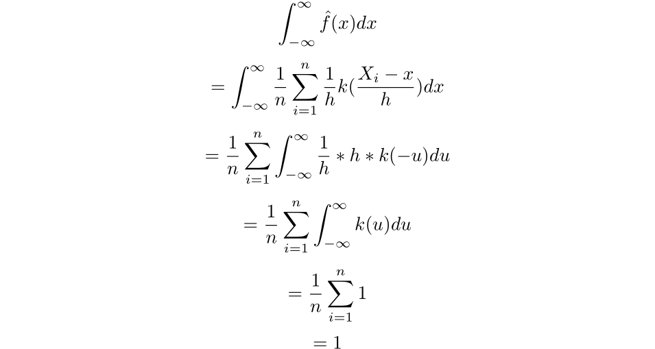
The first fact that we will need to utilize is that the integral of the estimator across the real line is 1. To prove this fact, we will need to make use of the change of u-substitution:

Employing that u-substitution we get the following:

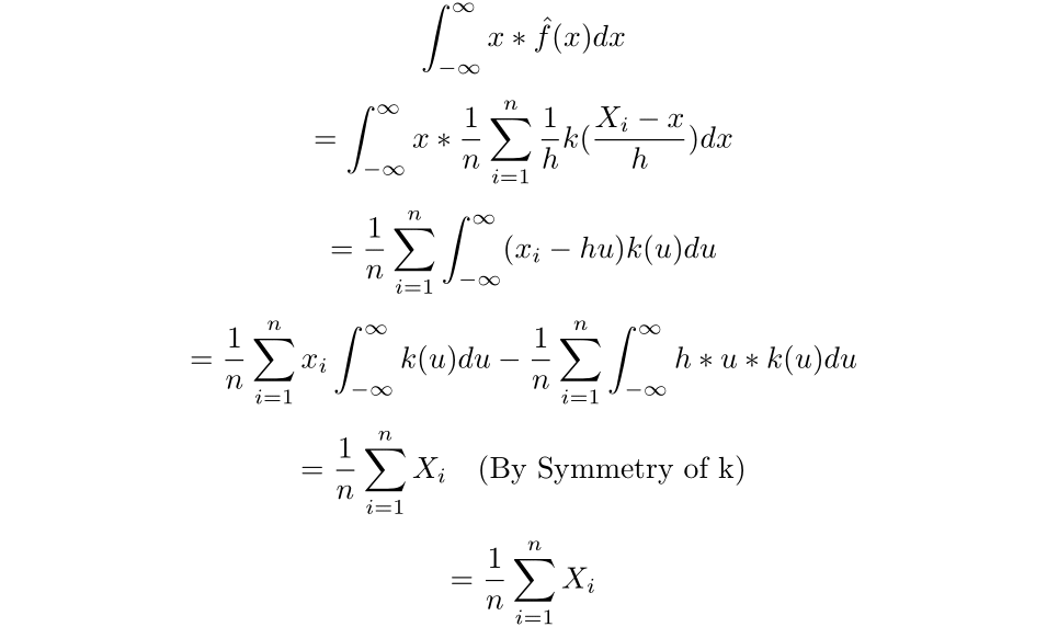
Now we can find the mean of the estimated density:

Therefore, the mean of the estimated density is simply the sample mean.

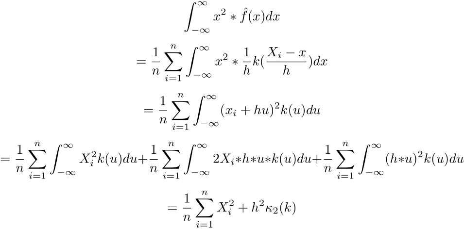
Now let us find the second moment of the estimator.

We can then find the variance of the estimated density:

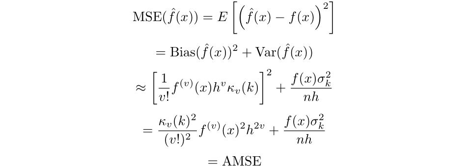
To find the optimal bandwidth and kernel, we will be minimizing the mean squared error of the estimator. To achieve this, we will first need to find the bias and variance of the estimator.

The expected value of a random variable, X, with a probability density function of f, can be calculated as:

Thus,

Where z is a dummy variable of integration. We can then use a change of variables to get the following:

Therefore, we get the following:

Most of the time, however, the integral above is not analytically solvable. Therefore, we will have to approximate f(x+ hu) by using its Taylor expansion. As a reminder, the Taylor expansion of f(x) around a is:

Thus, assume f(x) is differentiable to the v+1 term. For f(x+hu) the expansion is:

Then for a v-order kernel, we can take the expression out to the v’th term:

Where the last term is the remainder, which vanishes faster than h as h approaches 0. Now, assuming that k is a v’th order kernel function, we have that:

Therefore:

Thus we have that the bias of the estimator is then:

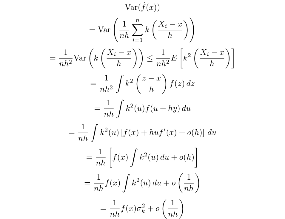
The upper bound for the variance can be obtained via the following calculation [Chen 2].

Where:

This term is also known as the roughness and can be denoted as R(k).

Finally, we can get an expression for the mean squared error:

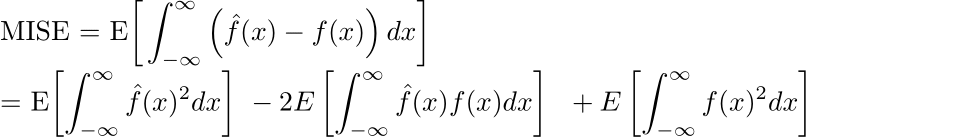
Where AMSE is short for asymptotic mean squared error. We can then minimize the asymptotic mean integrated square error defined as follows,

to find what bandwidth will lead to the lowest error (Silverman, 1986):

Then, by setting the equation to 0 and simplifying we find that the optimal bandwidth for a kernel of order v is:

The more familiar expression is for second order kernels, where the bandwidth that minimizes the AMISE is:

However, this solution may be a letdown as we require knowing the distribution that we are estimating to find the optimal bandwidth. In practice, we would not have this distribution if we were using the kernel density estimator in the first place.

Part 4: Bandwidth Selection

Despite not being able to find the bandwidth that minimizes the mean integrated square error, there are several methods available to choose a bandwidth without knowing the underlying distribution. It is important to note, however, that a larger h value will cause your estimator to have less variance but greater bias, while a smaller bandwidth will produce a rougher estimate with less bias (Eidous et al., 2010).

Some methods to find a bandwidth include using:

1: The Solve-the-Equation Rule

2: Least Squares Cross-Validation

3: Biased Cross-Validation

4: The Direct Plug in Method

5: The Contrast Method

It is important to note that depending on the sample size and skewness of your data, the ‘best’ method to choose your bandwidth changes. Most packages in Python allow you to use Silverman’s proposed method, where you directly plug in some distribution (typically normal) for f and then compute the bandwidth based upon the kernel function that you have chosen. This procedure, known as Silverman’s Rule of Thumb, provides a relatively simple estimate for the bandwidth. However, it often tends to overestimate, resulting in a smoother estimate with lower variance but higher bias. Silverman’s Rule of Thumb also specifically does not perform well for bimodal distributions, and there are more accurate techniques available for those cases.

If you assume that your data is normally distributed with a mean of 0, use the sample standard deviation, and apply the Epanechnikov kernel (discussed below), you can select the bandwidth using the Rule of Thumb via the following equation:

Eidous et al. found the Contrast Method to have the best performance compared to the other methods I listed. However, this method has drawbacks, as it increases the number of parameters to be chosen.

The cross validation method is another good choice in bandwidth selection method, as it often leads to a small bias but a large variance (Heidenreich et al, 2013). It is most useful for when you are looking for a bandwidth selector that tends to undershoot the optimal bandwidth. To keep this article not overly long I will only be going over the Ordinary Least Squares Cross Validation method. The method tends to work well for rather wiggly densities and a moderate sample size of around 50 to 100. If you have a very small or large sample size this paper is a good resource to find another way to choose your bandwidth. As pointed out by Heidenreich, “it definitely makes a difference which bandwidth selector is chosen; not only in numerical terms but also for the quality of density estimation”.

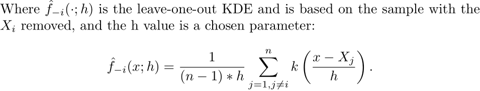
As a quick refresher, when we are creating a model we reserve some of our sample as a validation set to see how our model performs on the sample that it has not been trained on. K Fold Cross Validation minimizes the impact of possibly selecting a test set that misrepresents the dataset by splitting the dataset into K parts and then training the model K times and allowing each part to be the validation set once.

Leave One Out Cross Validation is K Fold Cross Validation taken to the extreme, where for a sample size of n, we train the model n times and leave out one sample each time. Here is an article that goes more in-depth into the method in the context of training machine learning algorithms.

Let us turn back to the AMISE expression. Instead of investigating the asymptotic mean integrated square error, we will minimize the mean integrated square error (MISE). First, we can expand the square:

As we have no control over the expected value of the last term, we can seek to minimize the first two terms and drop the third. Then, because X is an unbiased estimator for E[X], we can find the first term directly:

Then the convolution of k with k is defined as the following:

Hence,

Thus, for the first term, we have:

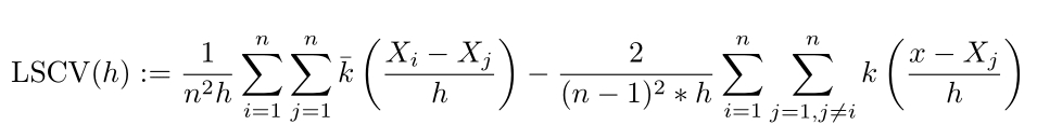
Next, we can approximate the second term by Monte Carlo methods. First, as discussed earlier, the density function is equivalent to the derivative of the cumulative distribution function, which we can approximate via the empirical distribution function. Then, the integral can be approximated by the average value of the estimator over the sample.

Then the least squares cross validation selector (LSCV) is defined as the following:

We then get the final selector defined as:

The optimal bandwidth is the h value that minimizes LSCV, defined as the following:

The LSCV(h) function can have multiple local minimums, hence the optimal bandwidth that you find can be sensitive to the interval chosen. It is useful to graph the function and then visually investigate where the global minimum lies.

Part 5: Optimal Kernel Selection

If we are working with a second order kernel (which is typical), the choice in kernel selection is much more straightforward than bandwidth. Under the criteria of minimizing the AMISE, the Epanechnikov kernel is an optimal kernel. The full proof can be found in this paper by Muler.

There are other kernels which are as efficient as the Epanechnikov kernel, which are also touched on in Muler’s paper. However, I wouldn’t worry too much about your choice of kernel function, the choice in bandwidth is much more important.

Part 6: Further Topics and Conclusion

Adaptive Bandwidths

One of the proposed ways to improve the Kernel Density Estimator is through an adaptive bandwidth. An adaptive bandwidth adjusts the bandwidth for each data point, increasing it when the density of the sample data is lower and decreasing it when the density is higher. While promising in theory, an adaptive bandwidth has been shown to perform quite poorly in the univariate case (Terrel, Scott 1992). While it may be better for larger dimensional spaces, for the one-dimensional case I believe it is best to stick with a constant bandwidth.

Multivariate Kernel Density Estimation

The kernel density estimator can also be extended to higher dimensions, where the kernel is a radial basis function or is a product of multiple kernel functions. The approach does suffer from the curse of dimensionality, where as the dimension grows larger the number of data points needed to produce a useful estimator grows exponentially. It is also computationally expensive and is not a great method for analyzing high-dimensional data.

Nonparametric multivariate density estimation is still a very active field, with Masked Autoregressive Flow appearing to be quite a new and promising approach.

Real World Applications

Kernel density estimation has numerous applications across disciplines. First, it has been shown to improve machine learning algorithms such as in the case of the flexible naive Bayes classifier.

It has also been used to estimate traffic accident density. The linked paper uses the KDE to help make a model that indicates the risk of traffic accidents in different cities across Japan.

Another fun use is in seismology, where the KDE has been used for modelling the risk of earthquakes in different locations.

Conclusion

The kernel density estimator is an excellent addition to the data analysts’ toolbox. While a histogram is certainly a fine way of analyzing data without using any underlying assumptions, the kernel density estimator provides a solid alternative for univariate data. For higher dimensional data, or for when computational time is a concern, I would recommend looking elsewhere. Nonetheless, the KDE is an intuitive, powerful and versatile tool in data analysis.

Unless otherwise noted, all images are by the author.

The Math Behind Kernel Density Estimation was originally published in Towards Data Science on Medium, where people are continuing the conversation by highlighting and responding to this story.