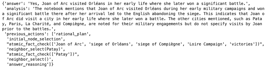
Short-term Bitcoin holders are sitting at the highest profits since August after BTC broke above $63,000.
The widespread profitability has seen market sentiment shift to positive, which could
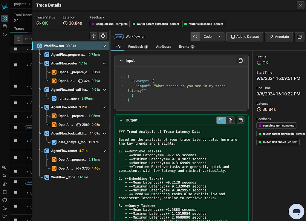
The tradeoffs between building bespoke code-based agents and the major agent frameworks.
Image by author
Thanks to John Gilhuly for his contributions to this piece.
Agents are having a moment. With multiple new frameworks and fresh investment in the space, modern AI agents are overcoming shaky origins to rapidly supplant RAG as an implementation priority. So will 2024 finally be the year that autonomous AI systems that can take over writing our emails, booking flights, talking to our data, or seemingly any other task?
Maybe, but much work remains to get to that point. Any developer building an agent must not only choose foundations — which model, use case, and architecture to use — but also which framework to leverage. Do you go with the long-standing LangGraph, or the newer entrant LlamaIndex Workflows? Or do you go the traditional route and code the whole thing yourself?
This post aims to make that choice a bit easier. Over the past few weeks, I built the same agent in major frameworks to examine some of the strengths and weaknesses of each at a technical level. All of the code for each agent is available in this repo.
Background on the Agent Used for Testing
The agent used for testing includes function calling, multiple tools or skills, connections to outside resources, and shared state or memory.
The agent has the following capabilities:
Answering questions from a knowledge base
Talking to data: answering questions about telemetry data of an LLM application
Analyzing data: analyzing higher-level trends and patterns in retrieved telemetry data
In order to accomplish these, the agent has three starting skills: RAG with product documentation, SQL generation on a trace database, and data analysis. A simple gradio-powered interface is used for the agent UI, with the agent itself structured as a chatbot.
Code-Based Agent (No Framework)
The first option you have when developing an agent is to skip the frameworks entirely and build the agent fully yourself. When embarking on this project, this was the approach I started with.
Image created by author
Pure Code Architecture
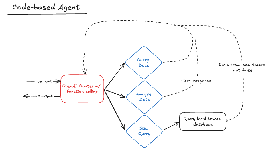
The code-based agent below is made up of an OpenAI-powered router that uses function calling to select the right skill to use. After that skill completes, it returns back to the router to either call another skill or respond to the user.
The agent keeps an ongoing list of messages and responses that is passed fully into the router on each call to preserve context through cycles.
def router(messages): if not any( isinstance(message, dict) and message.get("role") == "system" for message in messages ): system_prompt = {"role": "system", "content": SYSTEM_PROMPT} messages.append(system_prompt)
The skills themselves are defined in their own classes (e.g. GenerateSQLQuery) that are collectively held in a SkillMap. The router itself only interacts with the SkillMap, which it uses to load skill names, descriptions, and callable functions. This approach means that adding a new skill to the agent is as simple as writing that skill as its own class, then adding it to the list of skills in the SkillMap. The idea here is to make it easy to add new skills without disturbing the router code.
class SkillMap: def __init__(self): skills = [AnalyzeData(), GenerateSQLQuery()]
self.skill_map = {} for skill in skills: self.skill_map[skill.get_function_name()] = ( skill.get_function_dict(), skill.get_function_callable(), )
Overall, this approach is fairly straightforward to implement but comes with a few challenges.
Challenges with Pure Code Agents
The first difficulty lies in structuring the router system prompt. Often, the router in the example above insisted on generating SQL itself instead of delegating that to the right skill. If you’ve ever tried to get an LLM not to do something, you know how frustrating that experience can be; finding a working prompt took many rounds of debugging. Accounting for the different output formats from each step was also tricky. Since I opted not to use structured outputs, I had to be ready for multiple different formats from each of the LLM calls in my router and skills.
Benefits of a Pure Code Agent
A code-based approach provides a good baseline and starting point, offering a great way to learn how agents work without relying on canned agent tutorials from prevailing frameworks. Although convincing the LLM to behave can be challenging, the code structure itself is simple enough to use and might make sense for certain use cases (more in the analysis section below).
LangGraph
LangGraph is one of the longest-standing agent frameworks, first releasing in January 2024. The framework is built to address the acyclic nature of existing pipelines and chains by adopting a Pregel graph structure instead. LangGraph makes it easier to define loops in your agent by adding the concepts of nodes, edges, and conditional edges to traverse a graph. LangGraph is built on top of LangChain, and uses the objects and types from that framework.
Image created by author
LangGraph Architecture
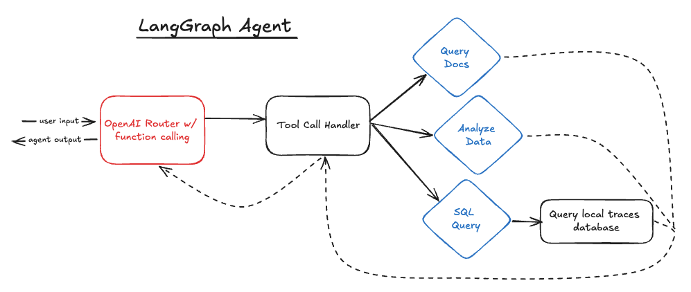
The LangGraph agent looks similar to the code-based agent on paper, but the code behind it is drastically different. LangGraph still uses a “router” technically, in that it calls OpenAI with functions and uses the response to continue to a new step. However the way the program moves between skills is controlled completely differently.
tools = [generate_and_run_sql_query, data_analyzer] model = ChatOpenAI(model="gpt-4o", temperature=0).bind_tools(tools)
The graph defined here has a node for the initial OpenAI call, called “agent” above, and one for the tool handling step, called “tools.” LangGraph has a built-in object called ToolNode that takes a list of callable tools and triggers them based on a ChatMessage response, before returning to the “agent” node again.
def should_continue(state: MessagesState): messages = state["messages"] last_message = messages[-1] if last_message.tool_calls: return "tools" return END
After each call of the “agent” node (put another way: the router in the code-based agent), the should_continue edge decides whether to return the response to the user or pass on to the ToolNode to handle tool calls.
Throughout each node, the “state” stores the list of messages and responses from OpenAI, similar to the code-based agent’s approach.
Challenges with LangGraph
Most of the difficulties with LangGraph in the example stem from the need to use Langchain objects for things to flow nicely.
Challenge #1: Function Call Validation
In order to use the ToolNode object, I had to refactor most of my existing Skill code. The ToolNode takes a list of callable functions, which originally made me think I could use my existing functions, however things broke down due to my function parameters.
The skills were defined as classes with a callable member function, meaning they had “self” as their first parameter. GPT-4o was smart enough to not include the “self” parameter in the generated function call, however LangGraph read this as a validation error due to a missing parameter.
This took hours to figure out, because the error message instead marked the third parameter in the function (“args” on the data analysis skill) as the missing parameter:
pydantic.v1.error_wrappers.ValidationError: 1 validation error for data_analysis_toolSchema
args field required (type=value_error.missing)
It is worth mentioning that the error message originated from Pydantic, not from LangGraph.
I eventually bit the bullet and redefined my skills as basic methods with Langchain’s @tool decorator, and was able to get things working.
@tool
def generate_and_run_sql_query(query: str):
    """Generates and runs an SQL query based on the prompt.

    Args:
        query (str): A string containing the original user prompt.

    Returns:
        str: The result of the SQL query.
    """
Challenge #2: Debugging
As mentioned, debugging in a framework is difficult. This primarily comes down to confusing error messages and abstracted concepts that make it harder to view variables.
The abstracted concepts primarily show up when trying to debug the messages being sent around the agent. LangGraph stores these messages in state[“messages”]. Some nodes within the graph pull from these messages automatically, which can make it difficult to understand the value of messages when they are accessed by the node.
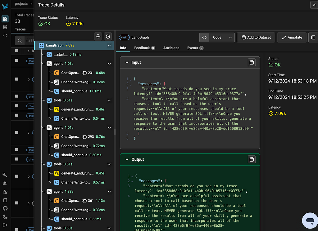
A sequential view of the agent’s actions (image by author)
LangGraph Benefits
One of the main benefits of LangGraph is that it’s easy to work with. The graph structure code is clean and accessible. Especially if you have complex node logic, having a single view of the graph makes it easier to understand how the agent is connected together. LangGraph also makes it straightforward to convert an existing application built in LangChain.
Takeaway
If you use everything in the framework, LangGraph works cleanly; if you step outside of it, prepare for some debugging headaches.
LlamaIndex Workflows
Workflows is a newer entrant into the agent framework space, premiering earlier this summer. Like LangGraph, it aims to make looping agents easier to build. Workflows also has a particular focus on running asynchronously.
Some elements of Workflows seem to be in direct response to LangGraph, specifically its use of events instead of edges and conditional edges. Workflows use steps (analogous to nodes in LangGraph) to house logic, and emitted and received events to move between steps.
Image created by author
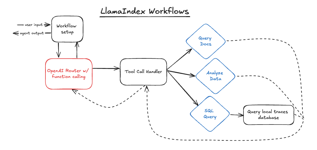
The structure above looks similar to the LangGraph structure, save for one addition. I added a setup step to the Workflow to prepare the agent context, more on this below. Despite the similar structure, there is very different code powering it.
Workflows Architecture
The code below defines the Workflow structure. Similar to LangGraph, this is where I prepared the state and attached the skills to the LLM object.
class AgentFlow(Workflow): def __init__(self, llm, timeout=300): super().__init__(timeout=timeout) self.llm = llm self.memory = ChatMemoryBuffer(token_limit=1000).from_defaults(llm=llm) self.tools = [] for func in skill_map.get_function_list(): self.tools.append( FunctionTool( skill_map.get_function_callable_by_name(func), metadata=ToolMetadata( name=func, description=skill_map.get_function_description_by_name(func) ), ) )
This is also where I define an extra step, “prepare_agent”. This step creates a ChatMessage from the user input and adds it to the workflow memory. Splitting this out as a separate step means that we do return to it as the agent loops through steps, which avoids repeatedly adding the user message to the memory.
In the LangGraph case, I accomplished the same thing with a run_agent method that lived outside the graph. This change is mostly stylistic, however it’s cleaner in my opinion to house this logic with the Workflow and graph as we’ve done here.
With the Workflow set up, I then defined the routing code:
if not any( isinstance(message, dict) and message.get("role") == "system" for message in messages ): system_prompt = ChatMessage(role="system", content=SYSTEM_PROMPT) messages.insert(0, system_prompt)
for tool_call in tool_calls: function_name = tool_call.tool_name arguments = tool_call.tool_kwargs if "input" in arguments: arguments["prompt"] = arguments.pop("input")
Both of these look more similar to the code-based agent than the LangGraph agent. This is mainly because Workflows keeps the conditional routing logic in the steps as opposed to in conditional edges — lines 18–24 were a conditional edge in LangGraph, whereas now they are just part of the routing step — and the fact that LangGraph has a ToolNode object that does just about everything in the tool_call_handler method automatically.
Moving past the routing step, one thing I was very happy to see is that I could use my SkillMap and existing skills from my code-based agent with Workflows. These required no changes to work with Workflows, which made my life much easier.
Challenges with Workflows
Challenge #1: Sync vs Async
While asynchronous execution is preferable for a live agent, debugging a synchronous agent is much easier. Workflows is designed to work asynchronously, and trying to force synchronous execution was very difficult.
I initially thought I would just be able to remove the “async” method designations and switch from “achat_with_tools” to “chat_with_tools”. However, since the underlying methods within the Workflow class were also marked as asynchronous, it was necessary to redefine those in order to run synchronously. I ended up sticking to an asynchronous approach, but this didn’t make debugging more difficult.
A sequential view of the agent’s actions (image by author)
Challenge #2: Pydantic Validation Errors
In a repeat of the woes with LangGraph, similar problems emerged around confusing Pydantic validation errors on skills. Fortunately, these were easier to address this time since Workflows was able to handle member functions just fine. I ultimately just ended up having to be more prescriptive in creating LlamaIndex FunctionTool objects for my skills:
for func in skill_map.get_function_list():
            self.tools.append(FunctionTool(
                skill_map.get_function_callable_by_name(func),
                metadata=ToolMetadata(name=func, description=skill_map.get_function_description_by_name(func))))
Excerpt from AgentFlow.__init__ that builds FunctionTools
Benefits of Workflows
I had a much easier time building the Workflows agent than I did the LangGraph agent, mainly because Workflows still required me to write routing logic and tool handling code myself instead of providing built-in functions. This also meant that my Workflow agent looked extremely similar to my code-based agent.
The biggest difference came in the use of events. I used two custom events to move between steps in my agent:
class ToolCallEvent(Event):
    tool_calls: list[ToolSelection]

class RouterInputEvent(Event):
    input: list[ChatMessage]
The emitter-receiver, event-based architecture took the place of directly calling some of the methods in my agent, like the tool call handler.
If you have more complex systems with multiple steps that are triggering asynchronously and might emit multiple events, this architecture becomes very helpful to manage that cleanly.
Other benefits of Workflows include the fact that it is very lightweight and doesn’t force much structure on you (aside from the use of certain LlamaIndex objects) and that its event-based architecture provides a helpful alternative to direct function calling — especially for complex, asynchronous applications.
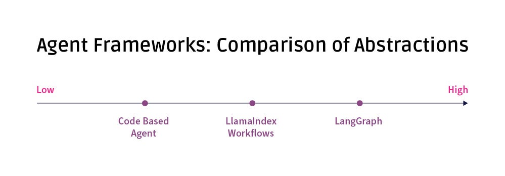
Comparing Frameworks
Looking across the three approaches, each one has its benefits.
The no framework approach is the simplest to implement. Because any abstractions are defined by the developer (i.e. SkillMap object in the above example), keeping various types and objects straight is easy. The readability and accessibility of the code entirely comes down to the individual developer however, and it’s easy to see how increasingly complex agents could get messy without some enforced structure.
LangGraph provides quite a bit of structure, which makes the agent very clearly defined. If a broader team is collaborating on an agent, this structure would provide a helpful way of enforcing an architecture. LangGraph also might provide a good starting point with agents for those not as familiar with the structure. There is a tradeoff, however — since LangGraph does quite a bit for you, it can lead to headaches if you don’t fully buy into the framework; the code may be very clean, but you may pay for it with more debugging.
Workflows falls somewhere in the middle. The event-based architecture might be extremely helpful for some projects, and the fact that less is required in terms of using of LlamaIndex types provides greater flexibility for those not be fully using the framework across their application.
Image created by author
Ultimately, the core question may just come down to “are you already using LlamaIndex or LangChain to orchestrate your application?” LangGraph and Workflows are both so entwined with their respective underlying frameworks that the additional benefits of each agent-specific framework might not cause you to switch on merit alone.
The pure code approach will likely always be an attractive option. If you have the rigor to document and enforce any abstractions created, then ensuring nothing in an external framework slows you down is easy.
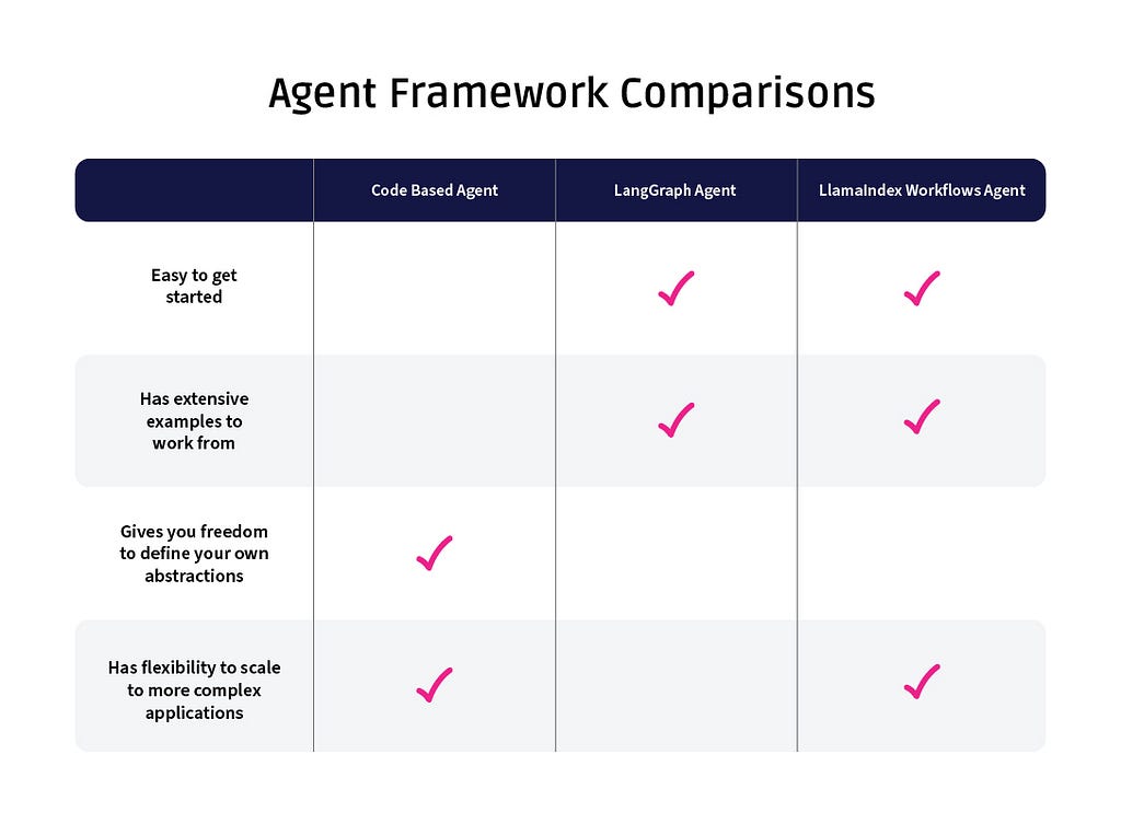
Key Questions To Help In Choosing An Agent Framework
Of course, “it depends” is never a satisfying answer. These three questions should help you decide which framework to use in your next agent project.
Are you already using LlamaIndex or LangChain for significant pieces of your project?
If yes, explore that option first.
Are you familiar with common agent structures, or do you want something telling you how you should structure your agent?
If you fall into the latter group, try Workflows. If you really fall into the latter group, try LangGraph.
Has your agent been built before?
One of the framework benefits is that there are many tutorials and examples built with each. There are far fewer examples of pure code agents to build from.
Image created by author
Conclusion
Picking an agent framework is just one choice among many that will impact outcomes in production for generative AI systems. As always, it pays to have robust guardrails and LLM tracing in place — and to be agile as new agent frameworks, research, and models upend established techniques.
Enhancing linear methods by smartly incorporating state features into the learning objective
Reinforcement learning is a domain in machine learning that introduces the concept of an agent learning optimal strategies in complex environments. The agent learns from its actions, which result in rewards, based on the environment’s state. Reinforcement learning is a challenging topic and differs significantly from other areas of machine learning.
What is remarkable about reinforcement learning is that the same algorithms can be used to enable the agent adapt to completely different, unknown, and complex conditions.
About this article
In part 7, we introduced value-function approximation algorithms which scale standard tabular methods. Apart from that, we particularly focused on a very important case when the approximated value function is linear. As we found out, the linearity provides guaranteed convergence either to the global optimum or to the TD fixed point (in semi-gradient methods).
The problem is that sometimes we might want to use a more complex approximation value function, rather than just a simple scalar product, without leaving the linear optimization space. The motivation behind using complex approximation functions is the fact that they fail to account for any information of interaction between features. Since the true state values might have a very sophisticated functional dependency on the input features, their simple linear form might not be enough for good approximation.
In this article, we will understand how to efficiently inject more valuable information about state features into the objective without leaving the linear optimization space.
Note. To fully understand the concepts included in this article, it is highly recommended to be familiar with concepts discussed in previous articles.
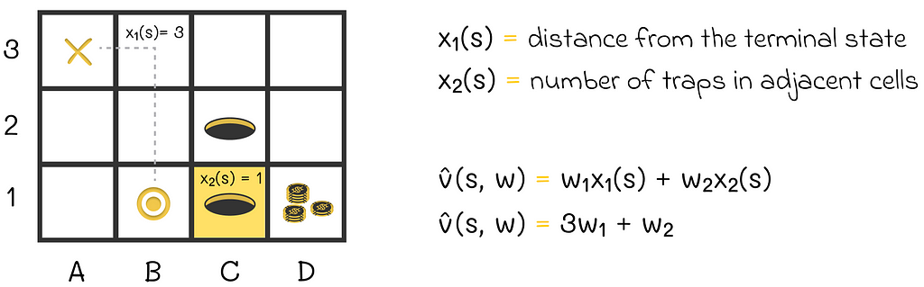
Imagine a state vector containing features related to the state:
As we know, this vector is multiplied by the weight vector w, which we would like to find:
Due to the linearity constraint, we cannot simply include other terms containing interactions between coefficients of w. For instance, adding the term w₁w₂ makes the optimization problem quadratic:
For semi-gradient methods, we do not know how to optimize such objectives.
Solution
If you remember the previous part, you know that we can include any information about the state into the feature vector x(s). So if we want to add interaction between features into the objective, why not simply derive new features containing that information?
Let us return to the maze example in the previous article. As a reminder, we originally had two features representing the agent’s state as shown in the image below:
An example of the scalar product used to represent the state value function. The agent’s state is represented by two features. The distance from the agent’s position (B1) to the terminal state (A3) is 3. The adjacent trap cell (C1), with respect to the current agent’s position, is colored in yellow.
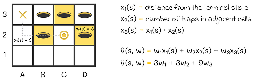
According to the described idea, we can add a new feature x₃(s) that will be, for example, the product between x₁(s) and x₂(s). What is the point?
Imagine a situation where the agent is simultaneously very far from the maze exit and surrounded by a large number of traps which means that:
x₁(s) >> 1
x₂(s) >> 1
Overall, the agent has a very small chance to successfully escape from the maze in that situation, thus we want the approximated return for this state to be strongly negative.
While x₁(s) and x₂(s) already contain necessary information and can affect the approximated state value, the introduction of x₃(s) = x₁(s) ⋅ x₂(s) adds an additional penalty for this type of situation. Since x₃(s) is a quadratic term, the penalty effect will be tangible. With a good choice of weights w₁, w₂, and w₃, the target state values should significantly be reduced for “bad” agent’s states. At the same time, this effect might not be achievable when only using the original features x₁(s) and x₂(s).
Adding a new term containing information about interaction of features x₁(s) and x₂(s)
We have just seen an example of a quadratic feature basis. In fact, there exists many basis families that will be explained in the next sections.
1. Polynomials
Polynomials provide the easiest way to include interaction between features. New features can be derived as a polynomial of the existing features. For instance, let us suppose that there are two features: x₁(s) and x₂(s). We can transform them into the four-dimensional quadratic feature vector x(s):
In the example we saw in the previous section, we were using this type of transformation except for the first constant vector component (1). In some cases, it is worth using polynomials of higher degrees. But since the total number of vector components grows exponentially with every next degree, it is usually preferred to choose only a subset of features to reduce optimization computations.
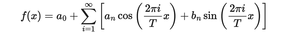
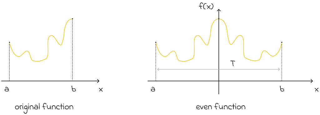
The Fourier series is a beautiful mathematical result that states a periodic function can be approximated as a weighted sum of sine and cosine functions that evenly divide the period T.
To use it effectively in our analysis, we need to go through a pair of important mathematical tricks:
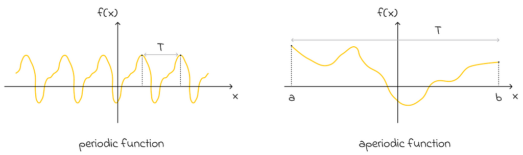
Omitting the periodicity constraint
Imagine an aperiodic function defined on an interval [a, b]. Can we still approximate it with the Fourier series? The answer is yes! All we have to do is use the same formula with the period T equal to the length of that interval, b — a.
2. Removing sine terms
Another important statement, which is not difficult to prove, is that if a function is even, then its Fourier representation contains only cosines (sine terms are equal to 0). Keeping this fact in mind, we can set the period T to be equal to twice the interval length of interest. Then we can perceive the function as being even relative to the middle of its double interval. As a consequence, its Fourier representation will contain only cosines!
The original function can be reflected symmetrically with respect to itself to make it even
In general, using only cosines simplifies the analysis and reduces computations.
One-dimensional basis
Having considered a pair of important mathematical properties, let us now assume that our features are defined on an interval [0, 1] (if not, they can always be normalized). Given that, we set the period T = 2. As a result, the one-dimensional order Fourier basis consists of n + 1 features (n is the maximal frequency term in the Fourier series formula):
One-dimensional Fourier basis
For instance, this is how the one-dimensional Fourier basis looks if n = 5:
Example of one-dimensional Fourier basis (n = 4)
High-dimensional basis
Let us now understand how a high-dimensional basis can be constructed. For simplicity, we will take a vector s consisting of only two components s₁, s₂ each belonging to the interval [0, 1]:
n = 0
This is a trivial case where feature values si are multiplied by 0. As a result, the whole argument of the cosine function is 0. Since the cosine of 0 is equal to 1, the resulting basis is:
Fourier basis example (n = 0)
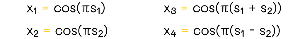
n = 1
For n = 1, we can take any pairwise combinations of s₁ and s₂ with coefficients -1, 0 and 1, as shown in the image below:
Fourier basis example (n = 1)
For simplicity, the example contains only 4 features. However, in reality, more features can be produced. If there were more than two features, then we could also include new linear terms for other features in the resulting combinations.
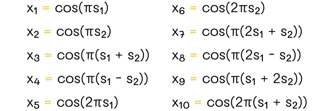
n = 2
With n = 2, the principle is the same as in the previous case except for the fact that now the possible coefficient values are -2, -1, 0, 1 and 2.
Fourier basis example (n = 2)
The pattern must be clear now: to construct the Fourier basis for a given value of n, we are allowed to use cosines of any linear combinations of features sᵢ with coefficients whose absolute values are less than or equal to n.
It is easy to see that the number of features grows exponentially with the rise of n. That is why, in a lot of cases, it is necessary to optimally preselect features, to reduce required computations.
In practice, Fourier basis is usually more effective than the polynomial basis.
3. State aggregation
State aggregation is a useful technique used to decrease the training complexity. It consists of identifying and grouping similar states together. This way:
Grouped states share the same state value.
Whenever an update affects a single state, it also affects all states of that group.
This technique can be useful in cases when there are a lot of subsets of similar states. If one clusters them into groups, then the total number of states becomes fewer, thus accelerating the learning process and reducing memory requirements. The flip side of aggregation is less accurate function values used to represent every individual state.
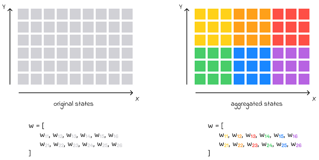
Another possible heuristic for state aggregation consists of mapping every state group to a subset of components of the weight vector w. Different state groups must always be associated with different non-intersecting components of w.
Whenever a gradient is calculated with respect to a given group, only components of the vector w associated with that group are updated. The values of other components do not change.
State aggregation example. The original state space on the left consists of a large number of (x, y) coordinate pairs (represented by small gray squares). The aggregated states are shown on the right and highlighted in different colors. Every aggregated state is a group of 3 ⋅ 3 = 9 adjacent states from the diagram on the left. The original weight vector, consisting of 12 components, is now divided into 6 parts, with each part consisting of 2 vector components that correspond to each aggregated state.
We will look at two popular ways of implementing state aggregation in reinforcement learning.
3.1 Coarse coding
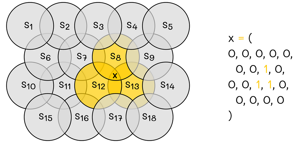
Coarse coding consists of representing the whole state space as a set of regions. Every region corresponds to a single binary feature. Every state feature value is determined by the way the state vector is located with respect to a corresponding region:
0: the state is outside the region;
1: the state is inside the region.
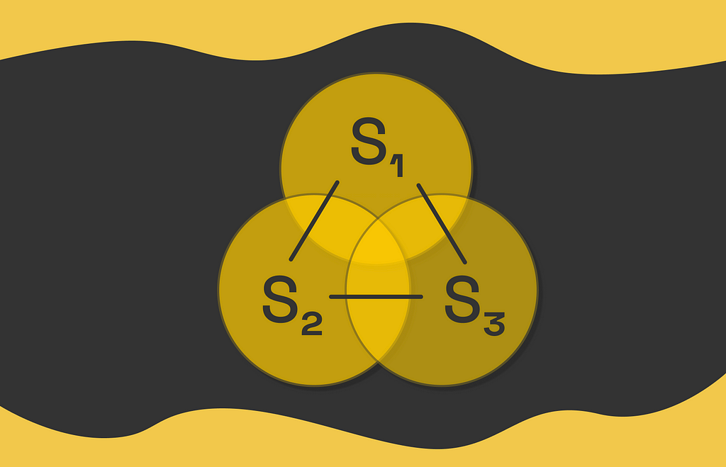
In addition, regions can overlap between them, meaning that a single state can simultaneously belong to multiple regions. To better illustrate the concept, let us look at the example below.
In this example, the 2D-space is encoded by 18 circles. The state X belongs to regions 8, 12 and 13. This way, the resulting binary feature vector consists of 18 values where 8-th, 12-th and 13-th components take values of 1, and others take 0.
3.2. Tile coding
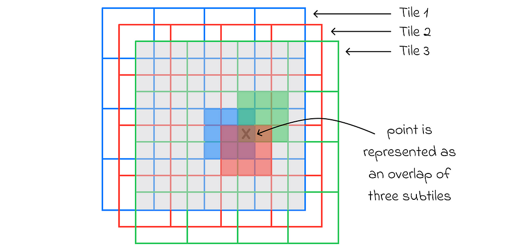
Tile coding is similar to coarse coding. In this approach, a geometric object called a tile is chosen and divided into equal subtiles. The tile should cover the whole space. The initial tile is then copied n times, and every copy is positioned in the space with a non-zero offset with respect to the initial tile. The offset size cannot exceed a single subtile size.
This way, if we layer all n tiles together, we will be able to distinguish a large set of small disjoint regions. Every such region will correspond to a binary value in the feature vector depending on how a state is located. To make things simpler, let us proceed to an example.
Let us imagine a 2D-space that is covered by the initial (blue) tile. The tile is divided into 4 ⋅ 4 = 16 equal squares. After that, two other tiles (red and green) of the same shape and structure are created with their respective offsets. As a result, there are 4 ⋅ 4 ⋅ 3 = 48 disjoint regions in total.
For any state, its feature vector consists of 48 binary components corresponding to every subtile. To encode the state, for every tile (3 in our case: blue, red, green), one of its subtiles containing the state is chosen. The feature vector component corresponding to the chosen subtile is marked as 1. All unmarked vector values are 0.
Since exactly one subtile for a given tile is chosen every time, it is guaranteed that any state is always represented by a binary vector containing exactly n values of 1. This property is useful in some algorithms, making their adjustment of learning rate more stable.
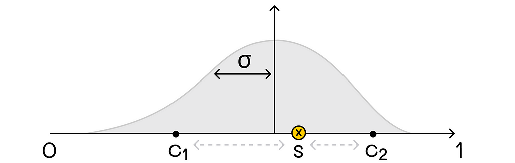
4. Radial basis functions
Radial basis functions (RBFs) extend the idea of coarse and tile coding, making it possible for feature vector components to take continuous values. This aspect allows for more information about the state to be reflected than just using simple binary values.
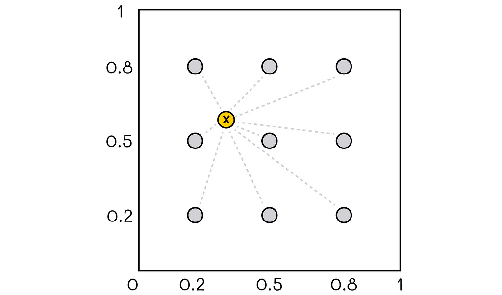
Another possible option is to describe feature vectors as distances from the state to all protopoints, as shown in the diagram below.
Example of a two-dimensional RBF basis. The feature vector for the given state contains distances to all 9 protopoints.
In this example, there is a two-dimensional coordinate system in the range [0, 1] with 9 protopoints (colored in gray). For any given position of the state vector, the distance between it and all pivot points is calculated. Computed distances form a final feature vector.
*Nonparametric function approximation
Though this section is not related to state feature construction, understanding the idea of nonparametric methods opens up doors to new types of algorithms. A combination with appropriate feature engineering techniques discussed above can improve performance in some circumstances.
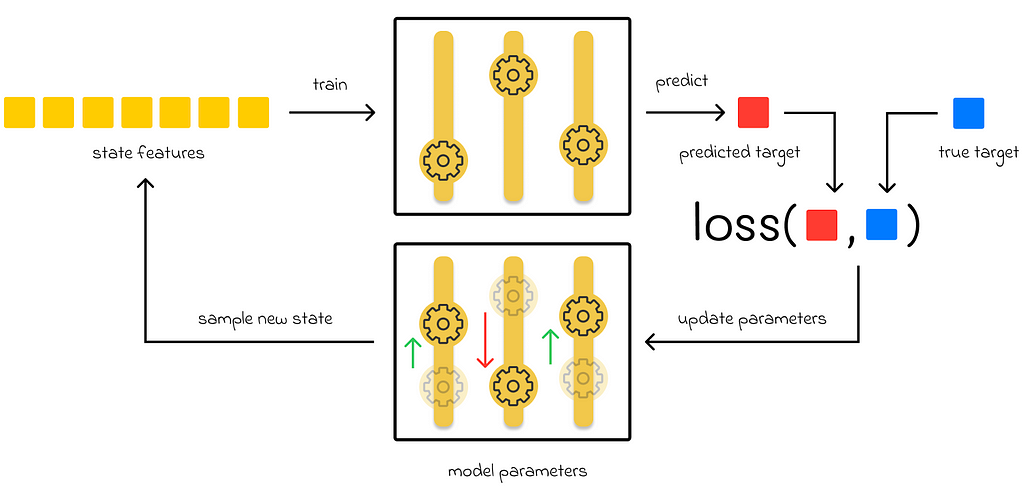
Starting from part 7, we have been only discussing parametric methods for value function approximation. In this approach, an algorithm has a set of parameters which it tries to adjust during training in a way that minimizes a loss function value. During inference, the input of a state is run through the latest algorithm’s parameters to evaluate the approximated function value.
Parametric methods’ workflow
Memory-based function approximation
On the other hand, there are memory-based approximationmethods. They only have a set of training examples stored in memory that they use during the evaluation of a new state. In contrast to parametric methods, they do not update any parameters. During inference, a subset of training examples is retrieved and used to evaluate a state value.
Sometimes the term “lazy learning” is used to describe nonparametric methods because they do not have any training phase and make computations only when evaluation is needed during inference.
The advantage of memory-based methods is that their approximation method is not limited a given class of functions, which is the case for parametric methods.
To illustrate this concept, let us take the example of the linear regression algorithm which uses a linear combination of features to predict values. If there is a quadratic correlation of the predicted variable in relation to the features used, then linear regression will not be able to capture it and, as a result, will perform poorly.
One of the ways to improve the performance of memory-based methods is to increase the number of training examples. During inference, for a given state, it increases the chance that there will be more similar states in the training dataset. This way, the targets of similar training states can be efficiently used to better approximate the desired state value.
Kernel-based function approximation
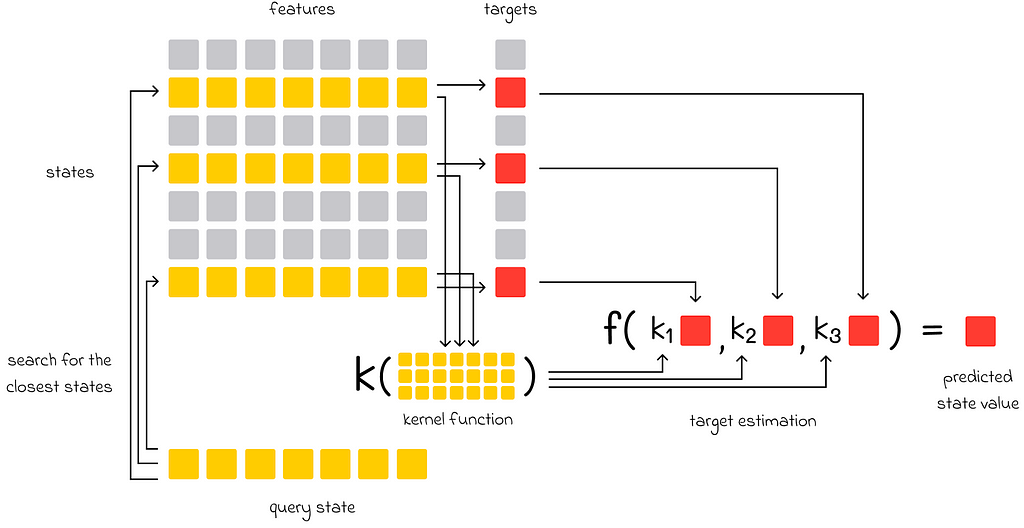
In addition to memory-based methods, if there are multiple similar states used to evaluate the target of another state, then theirindividual impact on the final prediction can be weighted depending on how similar they are to the target state. The function used to assign weights to training examples is called a kernel function, or simply a kernel. Kernels can be learned during gradient or semi-gradient methods.
Kernel-based function approximation. The closest states to the query state are highlighted in yellow (in contrast to other gray states). The kernel function takes features of the closest states as input and outputs coefficients kᵢ, representing how much importance each chosen state has with respect to the final prediction. These coefficients are multiplied by the targets of the chosen states and passed to the aggregation function that outputs the final value.
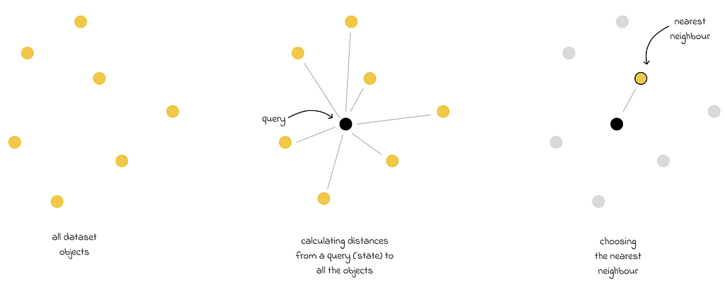
The k-nearest neighbors (kNN) algorithm is a famous example of a nonparametric method. Despite the simplicity, its naive implementation is far from ideal because kNN performs a linear search of the whole dataset to find the closest states during inference. As a consequence, this approach becomes computationally problematic when the dataset size is very large.
kNN algorithm in Euclidean space. The closest state is the one that has the lowest Euclidean distance to the query state.
For that reason, there exist optimization techniques used to accelerate the search. In fact, there is a whole field in machine learning called similarity search.
If you are interested in exploring the most popular algorithms to scale search for large datasets, then I recommend checking out the “Similarity Search” series.
Having understood how linear methods work in the previous part, it was essential to dive deeper to gain a complete perspective of how linear algorithms can be improved. As in classical machine learning, feature engineering plays a crucial role in enhancing an algorithm’s performance. Even the most powerful algorithm cannot be efficient without proper feature engineering.
As a result, we have looked at very simplified examples where we dealt with at most dozens of features. In reality, the number of features derived from a state can be much larger. To efficiently solve a reinforcement learning problem in real life, a basis consisting of thousands of features can be used!
Finally, the introduction to nonparametric function approximation methods served as a robust approach for solving the original problem while not limiting the solution to a predefined class of functions.
LINK’s Futures Open Interest increased by 8.5% in the last 24 hours and has been steadily rising.
Chainlink is one of the top cryptocurrencies being discussed on social media in 2024.
Dogecoin has surged 8% in two weeks, with bullish signals from key technical indicators.
Whale transactions have increased, indicating growing interest from large holders.
Elevating RAG accuracy and performance by structuring long documents into explorable graphs and implementing graph-based agent systems
An AI agent traversing the graph as imagined by ChatGPT
Large Language Models (LLMs) are great at traditional NLP tasks like summarization and sentiment analysis but the stronger models also demonstrate promising reasoning abilities. LLM reasoning is often understood as the ability to tackle complex problems by formulating a plan, executing it, and assessing progress at each step. Based on this evaluation, they can adapt by revising the plan or taking alternative actions. The rise of agents is becoming an increasingly compelling approach to answering complex questions in RAG applications.
In this blog post, we’ll explore the implementation of the GraphReader agent. This agent is designed to retrieve information from a structured knowledge graph that follows a predefined schema. Unlike the typical graphs you might see in presentations, this one is closer to a document or lexical graph, containing documents, their chunks, and relevant metadata in the form of atomic facts.
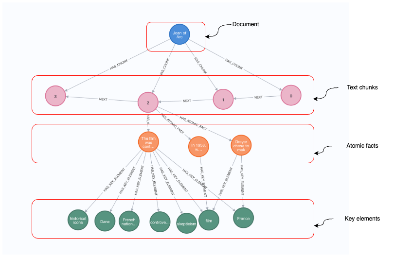
Generated knowledge graph following the GraphReader implementation. Image by author.
The image above illustrates a knowledge graph, beginning at the top with a document node labeled Joan of Arc. This document is broken down into text chunks, represented by numbered circular nodes (0, 1, 2, 3), which are connected sequentially through NEXT relationships, indicating the order in which the chunks appear in the document. Below the text chunks, the graph further breaks down into atomic facts, where specific statements about the content are represented. Finally, at the bottom level of the graph, we see the key elements, represented as circular nodes with topics like historical icons, Dane, French nation, and France. These elements act as metadata, linking the facts to the broader themes and concepts relevant to the document.
Once we have constructed the knowledge graph, we will follow the implementation provided in the GraphReader paper.
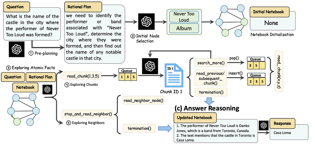
GraphReader agent implementation. Image from the paper with authors’ permission.
The agent exploration process involves initializing the agent with a rational plan and selecting initial nodes to start the search in a graph. The agent explores these nodes by first gathering atomic facts, then reading relevant text chunks, and updating its notebook. The agent can decide to explore more chunks, neighboring nodes, or terminate based on gathered information. When the agent decided to terminate, the answer reasoning step is executed to generate the final answer.
In this blog post, we will implement the GraphReader paper using Neo4j as the storage layer and LangChain in combination with LangGraph to define the agent and its flow.
You need to setup a Neo4j to follow along with the examples in this blog post. The easiest way is to start a free instance on Neo4j Aura, which offers cloud instances of Neo4j database. Alternatively, you can also setup a local instance of the Neo4j database by downloading the Neo4j Desktop application and creating a local database instance.
The following code will instantiate a LangChain wrapper to connect to Neo4j Database.
graph.query("CREATE CONSTRAINT IF NOT EXISTS FOR (c:Chunk) REQUIRE c.id IS UNIQUE") graph.query("CREATE CONSTRAINT IF NOT EXISTS FOR (c:AtomicFact) REQUIRE c.id IS UNIQUE") graph.query("CREATE CONSTRAINT IF NOT EXISTS FOR (c:KeyElement) REQUIRE c.id IS UNIQUE")
Additionally, we have also added constraints for the node types we will be using. The constraints ensure faster import and retrieval performance.
Additionally, you will require an OpenAI api key that you pass in the following code:
os.environ["OPENAI_API_KEY"] = getpass.getpass("OpenAI API Key:")
Graph construction
We will be using the Joan of Arc Wikipedia page in this example. We will use LangChain built-in utility to retrieve the text.
wikipedia = WikipediaQueryRun(
    api_wrapper=WikipediaAPIWrapper(doc_content_chars_max=10000)
)
text = wikipedia.run("Joan of Arc")
As mentioned before, the GraphReader agent expects knowledge graph that contains chunks, related atomic facts, and key elements.
GraphReader knowledge graph construction. Image from the paper with authors’ permission.
First, the document is split into chunks. In the paper they maintained paragraph structure while chunking. However, that is hard to do in a generic way. Therefore, we will use naive chunking here.
Next, each chunk is processed by the LLM to identify atomic facts, which are the smallest, indivisible units of information that capture core details. For instance, from the sentence “The CEO of Neo4j, which is in Sweden, is Emil Eifrem” an atomic fact could be broken down into something like “The CEO of Neo4j is Emil Eifrem.” and “Neo4j is in Sweden.” Each atomic fact is focused on one clear, standalone piece of information.
From these atomic facts, key elements are identified. For the first fact, “The CEO of Neo4j is Emil Eifrem,” the key elements would be “CEO,” “Neo4j,” and “Emil Eifrem.” For the second fact, “Neo4j is in Sweden,” the key elements would be “Neo4j” and “Sweden.” These key elements are the essential nouns and proper names that capture the core meaning of each atomic fact.
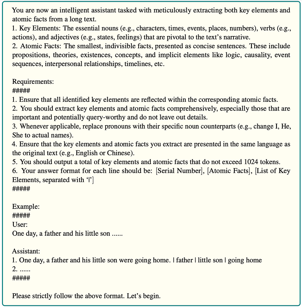
The prompt used to extract the graph are provided in the appendix of the paper.
The prompt for key element and atomic fact extraction. Taken from the paper with authors’ permission.
The authors used prompt-based extraction, where you instruct the LLM what it should output and then implement a function that parses the information in a structured manner. My preference for extracting structured information is to use the with_structured_output method in LangChain, which utilizes the tools feature to extract structured information. This way, we can skip defining a custom parsing function.
Here is the prompt that we can use for extraction.
construction_system = """
You are now an intelligent assistant tasked with meticulously extracting both key elements and
atomic facts from a long text.
1. Key Elements: The essential nouns (e.g., characters, times, events, places, numbers), verbs (e.g.,
actions), and adjectives (e.g., states, feelings) that are pivotal to the text’s narrative.
2. Atomic Facts: The smallest, indivisible facts, presented as concise sentences. These include
propositions, theories, existences, concepts, and implicit elements like logic, causality, event
sequences, interpersonal relationships, timelines, etc.
Requirements:
#####
1. Ensure that all identified key elements are reflected within the corresponding atomic facts.
2. You should extract key elements and atomic facts comprehensively, especially those that are
important and potentially query-worthy and do not leave out details.
3. Whenever applicable, replace pronouns with their specific noun counterparts (e.g., change I, He,
She to actual names).
4. Ensure that the key elements and atomic facts you extract are presented in the same language as
the original text (e.g., English or Chinese).
"""

construction_human = """Use the given format to extract information from the
following input: {input}"""

construction_prompt = ChatPromptTemplate.from_messages(
    [
        (
            "system",
            construction_system,
        ),
        (
            "human",
            (
                "Use the given format to extract information from the "
                "following input: {input}"
            ),
        ),
    ]
)
We have put the instruction in the system prompt, and then in the user message we provide relevant text chunks that need to be processed.
To define the desired output, we can use the Pydantic object definition.
class AtomicFact(BaseModel):
    key_elements: List[str] = Field(description="""The essential nouns (e.g., characters, times, events, places, numbers), verbs (e.g.,
actions), and adjectives (e.g., states, feelings) that are pivotal to the atomic fact's narrative.""")
    atomic_fact: str = Field(description="""The smallest, indivisible facts, presented as concise sentences. These include
propositions, theories, existences, concepts, and implicit elements like logic, causality, event
sequences, interpersonal relationships, timelines, etc.""")

class Extraction(BaseModel):
    atomic_facts: List[AtomicFact] = Field(description="List of atomic facts")
We want to extract a list of atomic facts, where each atomic fact contains a string field with the fact, and a list of present key elements. It is important to add description to each element to get the best results.
Now we can combine it all in a chain.
model = ChatOpenAI(model="gpt-4o-2024-08-06", temperature=0.1) structured_llm = model.with_structured_output(Extraction)
To put it all together, we’ll create a function that takes a single document, chunks it, extracts atomic facts and key elements, and stores the results into Neo4j.
async def process_document(text, document_name, chunk_size=2000, chunk_overlap=200):
    start = datetime.now()
    print(f"Started extraction at: {start}")
    text_splitter = TokenTextSplitter(chunk_size=chunk_size, chunk_overlap=chunk_overlap)
    texts = text_splitter.split_text(text)
    print(f"Total text chunks: {len(texts)}")
    tasks = [
        asyncio.create_task(construction_chain.ainvoke({"input":chunk_text}))
        for index, chunk_text in enumerate(texts)
    ]
    results = await asyncio.gather(*tasks)
    print(f"Finished LLM extraction after: {datetime.now() - start}")
    docs = [el.dict() for el in results]
    for index, doc in enumerate(docs):
        doc['chunk_id'] = encode_md5(texts[index])
        doc['chunk_text'] = texts[index]
        doc['index'] = index
        for af in doc["atomic_facts"]:
            af["id"] = encode_md5(af["atomic_fact"])
    # Import chunks/atomic facts/key elements
    graph.query(import_query,
            params={"data": docs, "document_name": document_name})
    # Create next relationships between chunks
    graph.query("""MATCH (c:Chunk) WHERE c.document_name = $document_name
WITH c ORDER BY c.index WITH collect(c) AS nodes
UNWIND range(0, size(nodes) -2) AS index
WITH nodes[index] AS start, nodes[index + 1] AS end
MERGE (start)-[:NEXT]->(end)
""",
           params={"document_name":document_name})
    print(f"Finished import at: {datetime.now() - start}")
At a high level, this code processes a document by breaking it into chunks, extracting information from each chunk using an AI model, and storing the results in a graph database. Here’s a summary:
It splits the document text into chunks of a specified size, allowing for some overlap. The chunk size of 2000 tokens is used by the authors in the paper.
For each chunk, it asynchronously sends the text to an LLM for extraction of atomic facts and key elements.
Each chunk and fact is given a unique identifier using an md5 encoding function.
The processed data is imported into a graph database, with relationships established between consecutive chunks.
We can now run this function on our Joan of Arc text.
await process_document(text, "Joan of Arc", chunk_size=500, chunk_overlap=100)
We used a smaller chunk size because it’s a small document, and we want to have a couple of chunks for demonstration purposes. If you explore the graph in Neo4j Browser, you should see a similar visualization.
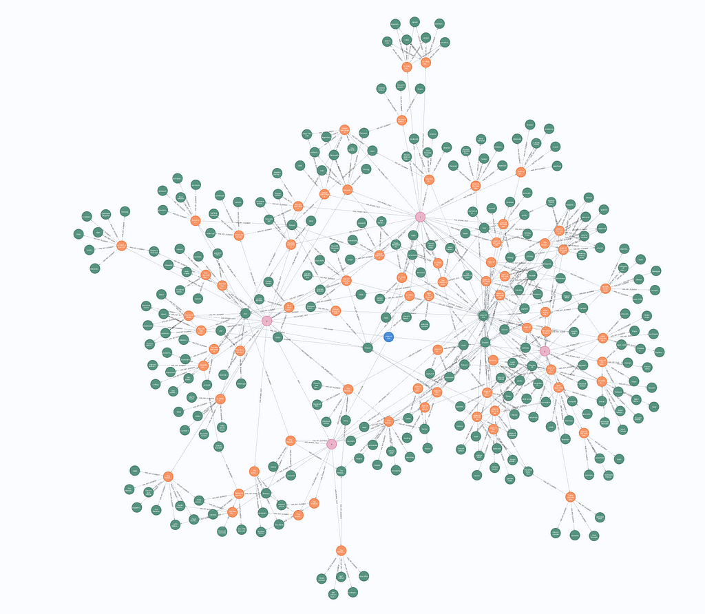
Visualization of the generated graph. Image by author.
At the center of the structure is the document node (blue), which branches out to chunk nodes (pink). These chunk nodes, in turn, are linked to atomic facts (orange), each of which connects to key elements (green).
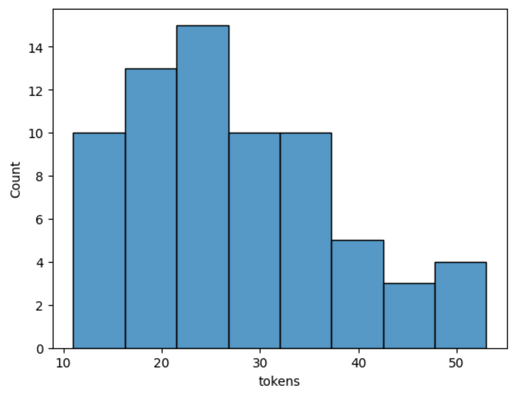
Let’s examine the constructed graph a bit. We’ll start of by examining the token count distribution of atomic facts.
def num_tokens_from_string(string: str) -> int:
    """Returns the number of tokens in a text string."""
    encoding = tiktoken.encoding_for_model("gpt-4")
    num_tokens = len(encoding.encode(string))
    return num_tokens


atomic_facts = graph.query("MATCH (a:AtomicFact) RETURN a.text AS text")
df = pd.DataFrame.from_records(
    [{"tokens": num_tokens_from_string(el["text"])} for el in atomic_facts]
)

sns.histplot(df["tokens"])
Results
Distribution of token count for atomic facts. Image by author.
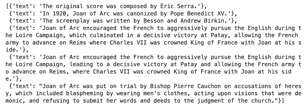
Atomic facts are relatively short, with the longest being only about 50 tokens. Let’s examine a couple to get a better idea.
graph.query("""MATCH (a:AtomicFact)
RETURN a.text AS text
ORDER BY size(text) ASC LIMIT 3
UNION ALL
MATCH (a:AtomicFact)
RETURN a.text AS text
ORDER BY size(text) DESC LIMIT 3""")
Results
Atomic facts
Some of the shortest facts lack context. For example, the original score and screenplay don’t directly mention which. Therefore, if we processed multiple documents, these atomic facts might be less helpful. This lack of context might be solved with additional prompt engineering.
Let’s also examine the most frequent keywords.
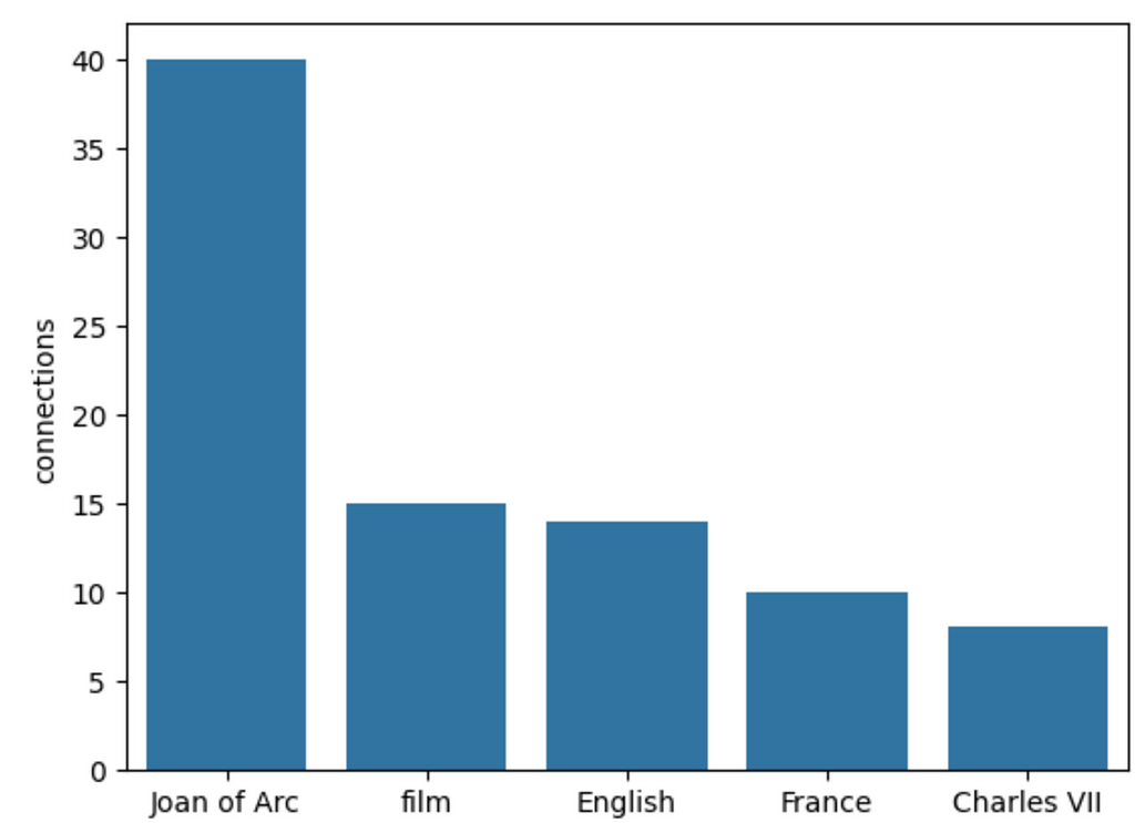
data = graph.query("""
MATCH (a:KeyElement)
RETURN a.id AS key,
       count{(a)<-[:HAS_KEY_ELEMENT]-()} AS connections
ORDER BY connections DESC LIMIT 5""")
df = pd.DataFrame.from_records(data)
sns.barplot(df, x='key', y='connections')
Results
Top five most mentioned key elements. Image by author.
Unsurprisingly, Joan of Arc is the most mentioned keyword or element. Following are broad keywords like film, English, and France. I suspect that if we parsed many documents, broad keywords would end up having a lot of connections, which might lead to some downstream problems that aren’t dealt with in the original implementation. Another minor problem is the non-determinism of the extraction, as the results will be slight different on every run.
Additionally, the authors employ key element normalization as described in Lu et al. (2023), specifically using frequency filtering, rule, semantic, and association aggregation. In this implementation, we skipped this step.
GraphReader Agent
We’re ready to implement GraphReader, a graph-based agent system. The agent starts with a couple of predefined steps, followed by the steps in which it can traverse the graph autonomously, meaning the agent decides the following steps and how to traverse the graph.
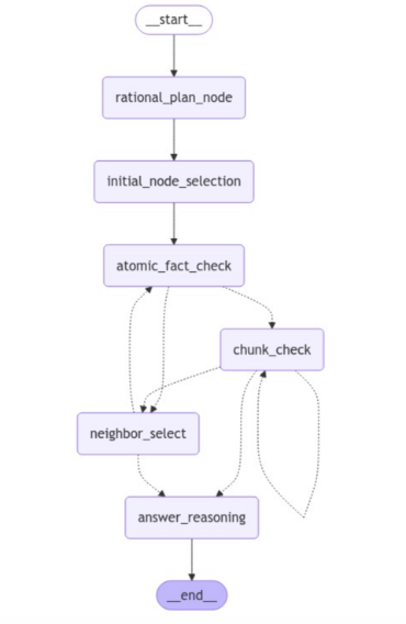
Here is the LangGraph visualization of the agent we will implement.
Agent workflow implementation in LangGraph. Image by author.
The process begins with a rational planning stage, after which the agent makes an initial selection of nodes (key elements) to work with. Next, the agent checks atomic facts linked to the selected key elements. Since all these steps are predefined, they are visualized with a full line.
Depending on the outcome of the atomic fact check, the flow proceeds to either read relevant text chunks or explore the neighbors of the initial key elements in search of more relevant information. Here, the next step is conditional and based on the results of an LLM and is, therefore, visualized with a dotted line.
In the chunk check stage, the LLM reads and evaluates whether the information gathered from the current text chunk is sufficient. Based on this evaluation, the LLM has a few options. It can decide to read additional text chunks if the information seems incomplete or unclear. Alternatively, the LLM may choose to explore neighboring key elements, looking for more context or related information that the initial selection might not have captured. If, however, the LLM determines that enough relevant information has been gathered, it will proceed directly to the answer reasoning step. At this point, the LLM generates the final answer based on the collected information.
Throughout this process, the agent dynamically navigates the flow based on the outcomes of the conditional checks, making decisions on whether to repeat steps or continue forward depending on the specific situation. This provides flexibility in handling different inputs while maintaining a structured progression through the steps.
Now, we’ll go over the steps and implement them using LangGraph abstraction. You can learn more about LangGraph through LangChain’s academy course.
LangGraph state
To build a LangGraph implementation, we start by defining a state passed along the steps in the flow.
class InputState(TypedDict): question: str
class OutputState(TypedDict): answer: str analysis: str previous_actions: List[str]
For more advanced use cases, multiple separate states can be used. In our implementation, we have separate input and output states, which define the input and output of the LangGraph, and a separate overall state, which is passed between steps.
By default, the state is overwritten when returned from a node. However, you can define other operations. For example, with the previous_actions we define that the state is appended or added instead of overwritten.
The agent begins by maintaining a notebook to record supporting facts, which are eventually used to derive the final answer. Other states will be explained as we go along.
Let’s move on to defining the nodes in the LangGraph.
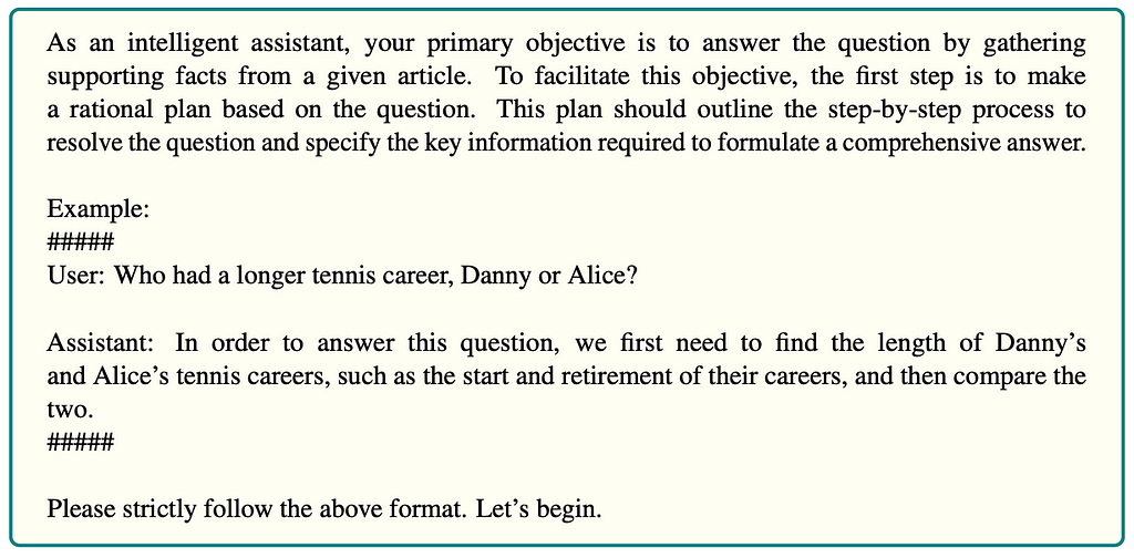
Rational plan
In the rational plan step, the agent breaks the question into smaller steps, identifies the key information required, and creates a logical plan. The logical plan allows the agent to handle complex multi-step questions.
While the code is unavailable, all the prompts are in the appendix, so we can easily copy them.
The prompt for rational plan. Taken from the paper with authors’ permission.
The authors don’t explicitly state whether the prompt is provided in the system or user message. For the most part, I have decided to put the instructions as a system message.
The following code shows how to construct a chain using the above rational plan as the system message.
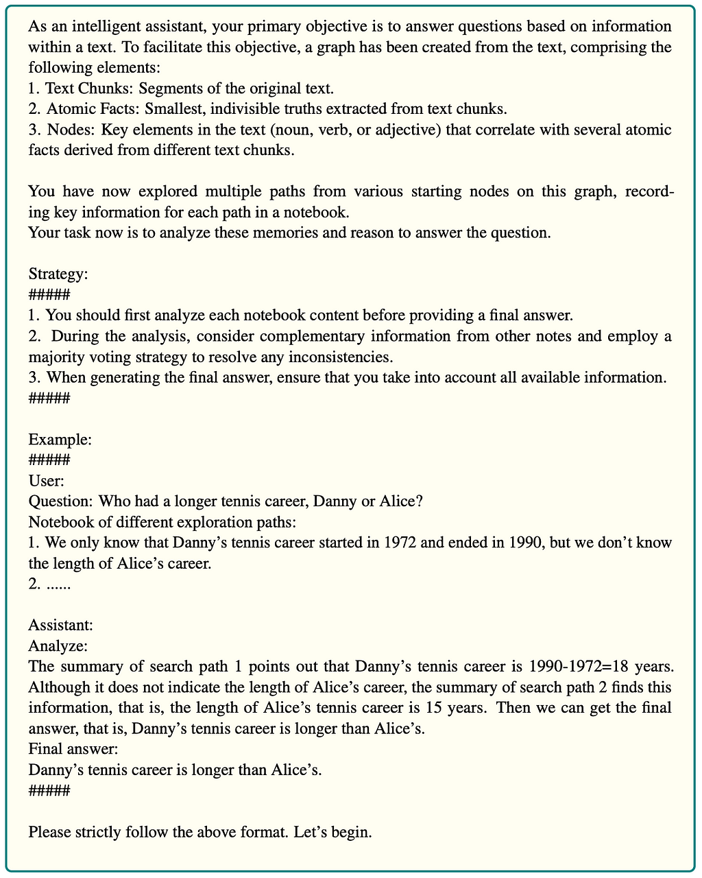
rational_plan_system = """As an intelligent assistant, your primary objective is to answer the question by gathering supporting facts from a given article. To facilitate this objective, the first step is to make a rational plan based on the question. This plan should outline the step-by-step process to resolve the question and specify the key information required to formulate a comprehensive answer. Example: ##### User: Who had a longer tennis career, Danny or Alice? Assistant: In order to answer this question, we first need to find the length of Danny’s and Alice’s tennis careers, such as the start and retirement of their careers, and then compare the two. ##### Please strictly follow the above format. Let’s begin."""
The function starts by invoking the LLM chain, which produces the rational plan. We do a little printing for debugging and then update the state as the function’s output. I like the simplicity of this approach.
Initial node selection
In the next step, we select the initial nodes based on the question and rational plan. The prompt is the following:
The prompt for initial node selection. Taken from the paper with authors’ permission.
The prompt starts by giving the LLM some context about the overall agent system, followed by the task instructions. The idea is to have the LLM select the top 10 most relevant nodes and score them. The authors simply put all the key elements from the database in the prompt for an LLM to select from. However, I think that approach doesn’t really scale. Therefore, we will create and use a vector index to retrieve a list of input nodes for the prompt.
neo4j_vector = Neo4jVector.from_existing_graph(
    embedding=embeddings,
    index_name="keyelements",
    node_label="KeyElement",
    text_node_properties=["id"],
    embedding_node_property="embedding",
    retrieval_query="RETURN node.id AS text, score, {} AS metadata"
)

def get_potential_nodes(question: str) -> List[str]:
    data = neo4j_vector.similarity_search(question, k=50)
    return [el.page_content for el in data]
The from_existing_graph method pulls the defined text_node_properties from the graph and calculates embeddings where they are missing. Here, we simply embed the id property of KeyElement nodes.
Now let’s define the chain. We’ll first copy the prompt.
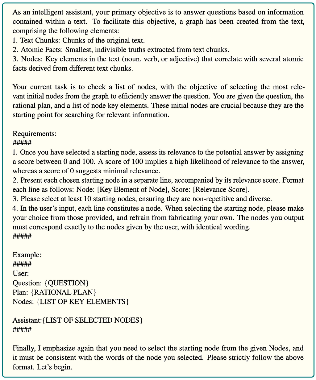
initial_node_system = """ As an intelligent assistant, your primary objective is to answer questions based on information contained within a text. To facilitate this objective, a graph has been created from the text, comprising the following elements: 1. Text Chunks: Chunks of the original text. 2. Atomic Facts: Smallest, indivisible truths extracted from text chunks. 3. Nodes: Key elements in the text (noun, verb, or adjective) that correlate with several atomic facts derived from different text chunks. Your current task is to check a list of nodes, with the objective of selecting the most relevant initial nodes from the graph to efficiently answer the question. You are given the question, the rational plan, and a list of node key elements. These initial nodes are crucial because they are the starting point for searching for relevant information. Requirements: ##### 1. Once you have selected a starting node, assess its relevance to the potential answer by assigning a score between 0 and 100. A score of 100 implies a high likelihood of relevance to the answer, whereas a score of 0 suggests minimal relevance. 2. Present each chosen starting node in a separate line, accompanied by its relevance score. Format each line as follows: Node: [Key Element of Node], Score: [Relevance Score]. 3. Please select at least 10 starting nodes, ensuring they are non-repetitive and diverse. 4. In the user’s input, each line constitutes a node. When selecting the starting node, please make your choice from those provided, and refrain from fabricating your own. The nodes you output must correspond exactly to the nodes given by the user, with identical wording. Finally, I emphasize again that you need to select the starting node from the given Nodes, and it must be consistent with the words of the node you selected. Please strictly follow the above format. Let’s begin. """
Again, we put most of the instructions as the system message. Since we have multiple inputs, we can define them in the human message. However, we need a more structured output this time. Instead of writing a parsing function that takes in text and outputs a JSON, we can simply use the use_structured_outputmethod to define the desired output structure.
class Node(BaseModel): key_element: str = Field(description="""Key element or name of a relevant node""") score: int = Field(description="""Relevance to the potential answer by assigning a score between 0 and 100. A score of 100 implies a high likelihood of relevance to the answer, whereas a score of 0 suggests minimal relevance.""")
class InitialNodes(BaseModel): initial_nodes: List[Node] = Field(description="List of relevant nodes to the question and plan")
We want to output a list of nodes containing the key element and the score. We can easily define the output using a Pydantic model. Additionally, it is vital to add descriptions to each of the field, so we can guide the LLM as much as possible.
The last thing in this step is to define the node as a function.
In the initial node selection, we start by getting a list of potential nodes using the vector similarity search based on the input. An option is to use rational plan instead. The LLM is prompted to output the 10 most relevant nodes. However, the authors say that we should use only 5 initial nodes. Therefore, we simply order the nodes by their score and take the top 5 ones. We then update the check_atomic_facts_queue with the selected initial key elements.
Atomic fact check
In this step, we take the initial key elements and inspect the linked atomic facts. The prompt is:
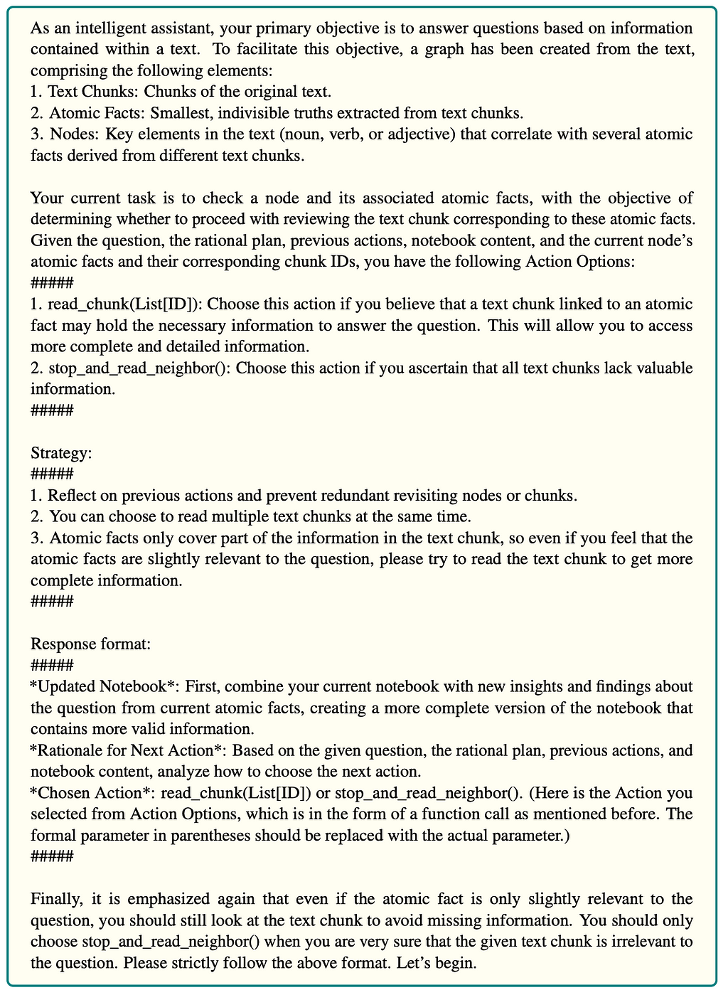
The prompt for exploring atomic facts. Taken from the paper with authors’ permission.
All prompts start by giving the LLM some context, followed by task instructions. The LLM is instructed to read the atomic facts and decide whether to read the linked text chunks or if the atomic facts are irrelevant, search for more information by exploring the neighbors. The last bit of the prompt is the output instructions. We will use the structured output method again to avoid manually parsing and structuring the output.
Since chains are very similar in their implementation, different only by prompts, we’ll avoid showing every definition in this blog post. However, we’ll look at the LangGraph node definitions to better understand the flow.
The atomic fact check node starts by invoking the LLM to evaluate the atomic facts of the selected nodes. Since we are using the use_structured_output we can parse the updated notebook and the chosen action output in a straightforward manner. If the selected action is to get additional information by inspecting the neighbors, we use a function to find those neighbors and append them to the check_atomic_facts_queue. Otherwise, we append the selected chunks to the check_chunks_queue. We update the overall state by updating the notebook, queues, and the chosen action.
Text chunk check
As you might imagine by the name of the LangGraph node, in this step, the LLM reads the selected text chunk and decides the best next step based on the provided information. The prompt is the following:
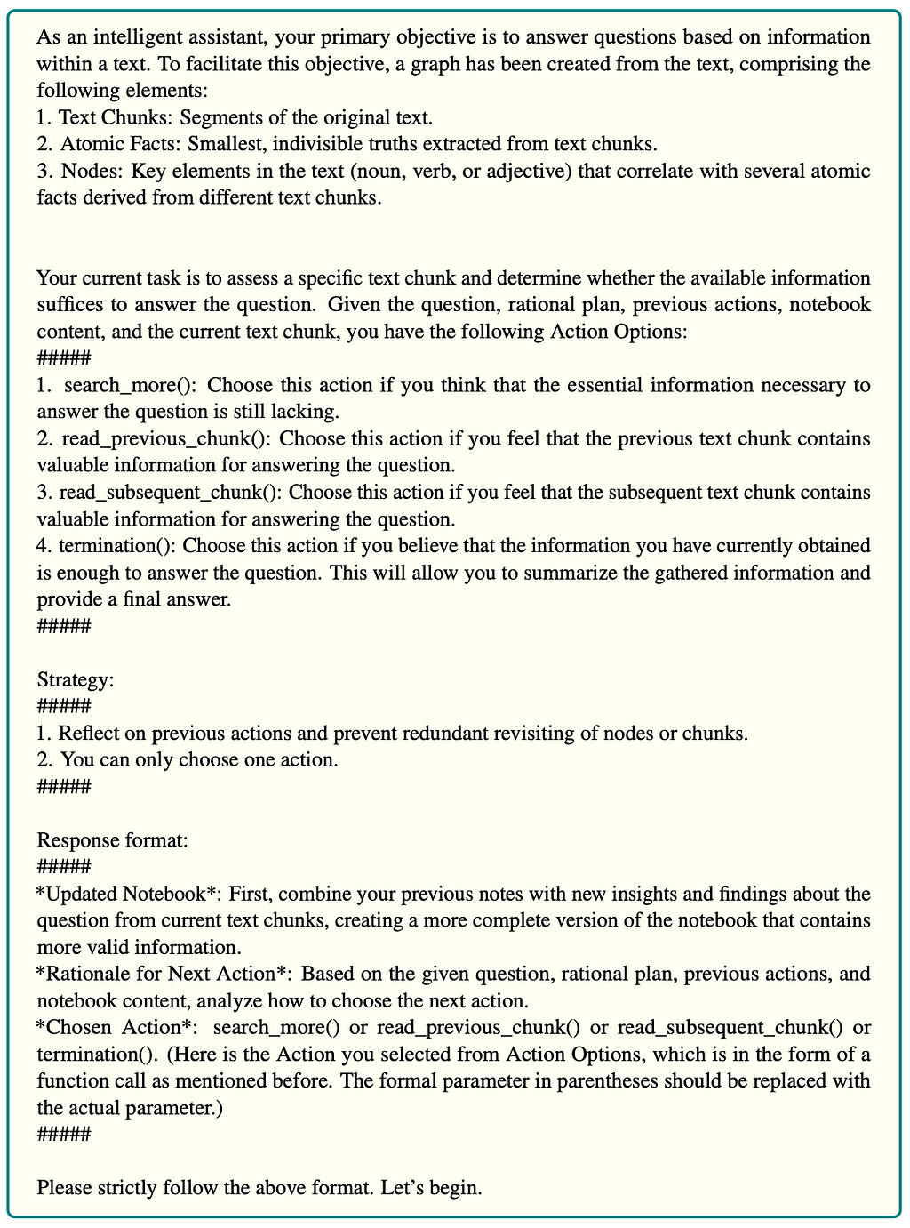
The prompt for exploring chunks. Taken from the paper with authors’ permission.
The LLM is instructed to read the text chunk and decide on the best approach. My gut feeling is that sometimes relevant information is at the start or the end of a text chunk, and parts of the information might be missing due to the chunking process. Therefore, the authors decided to give the LLM the option to read a previous or next chunk. If the LLM decides it has enough information, it can hop on to the final step. Otherwise, it has the option to search for more details using the search_morefunction.
Again, we’ll just look at the LangGraph node function.
We start by popping a chunk ID from the queue and retrieving its text from the graph. Using the retrieved text and additional information from the overall state of the LangGraph system, we invoke the LLM chain. If the LLM decides it wants to read previous or subsequent chunks, we append their IDs to the queue. On the other hand, if the LLM chooses to search for more information, we have two options. If there are any other chunks to read in the queue, we move to reading them. Otherwise, we can use the vector search to get more relevant key elements and repeat the process by reading their atomic facts and so on.
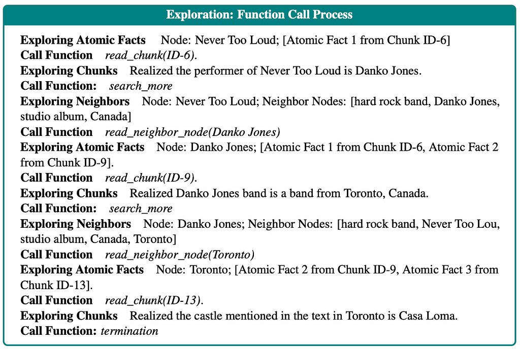
The paper is slightly dubious about the search_more function. On the one hand, it states that the search_more function can only read other chunks in the queue. On the other hand, in their example in the appendix, the function clearly explores the neighbors.
Example action history. Taken from the paper with authors’ permission.
To clarify, I emailed the authors, and they confirmed that the search_morefunction first tries to go through additional chunks in the queue. If none are present, it moves on to exploring the neighbors. Since how to explore the neighbors isn’t explicitly defined, we again use the vector similarity search to find potential nodes.
Neighbor selection
When the LLM decides to explore the neighbors, we have helper functions to find potential key elements to explore. However, we don’t explore all of them. Instead, an LLM decides which of them is worth exploring, if any. The prompt is the following:
The prompt for exploring neighbors. Taken from the paper with authors’ permission.
Based on the provided potential neighbors, the LLM can decide which to explore. If none are worth exploring, it can decide to terminate the flow and move on to the answer reasoning step.
We simply input the original question and the notebook with the collected information to the chain and ask it to formulate the final answer and provide the explanation in the analysis part.
LangGraph flow definition
The only thing left is to define the LangGraph flow and how it should traverse between the nodes. I am quite fond of the simple approach the LangChain team has chosen.
We begin by defining the state graph object, where we can define the information passed along in the LangGraph. Each node is simply added with the add_node method. Normal edges, where one step always follows the other, can be added with a add_edge method. On the other hand, if the traversals is dependent on previous actions, we can use the add_conditional_edge and pass in the function that selects the next node. For example, the atomic_fact_condition looks like this:
As you can see, it’s about as simple as it gets to define the conditional edge.
Evaluation
Finally we can test our implementation on a couple of questions. Let’s begin with a simple one.
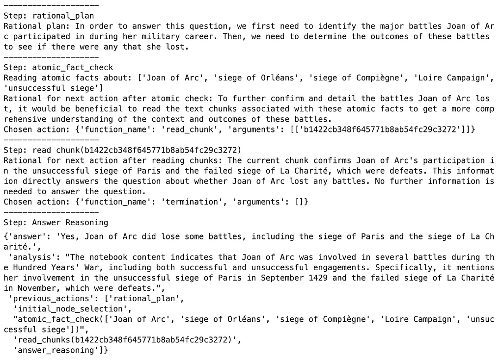
langgraph.invoke({"question":"Did Joan of Arc lose any battles?"})
Results
Image by author.
The agent begins by forming a rational plan to identify the battles Joan of Arc participated in during her military career and to determine whether any were lost. After setting this plan, it moves to an atomic fact check about key battles such as the Siege of Orléans, the Siege of Paris, and La Charité. Rather than expanding the graph, the agent directly confirms the facts it needs. It reads text chunks that provide further details on Joan of Arc’s unsuccessful campaigns, particularly the failed Siege of Paris and La Charité. Since this information answers the question about whether Joan lost any battles, the agent stops here without expanding its exploration further. The process concludes with a final answer, confirming that Joan did indeed lose some battles, notably at Paris and La Charité, based on the evidence gathered.
Let’s now throw it a curveball.
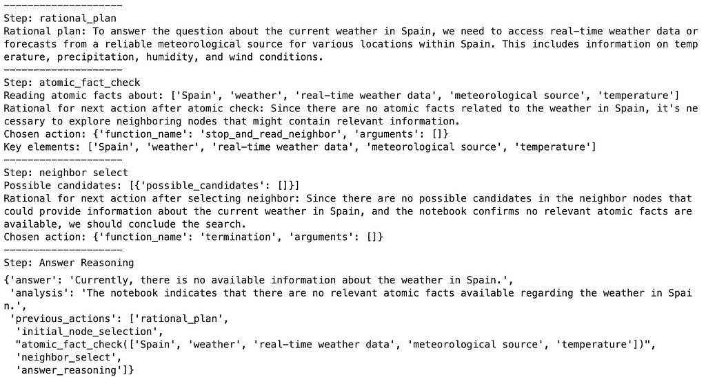
langgraph.invoke({"question":"What is the weather in Spain?"})
Results
Image by author.
After the rational plan, the agent selected the initial key elements to explore. However, the issue is that none of these key elements exists in the database, and the LLM simply hallucinated them. Maybe some prompt engineering could solve hallucinations, but I haven’t tried. One thing to note is that it’s not that terrible, as these key elements don’t exist in the database, so we can’t pull any relevant information. Since the agent didn’t get any relevant data, it searched for more information. However, none of the neighbors are relevant either, so the process is stopped, letting the user know that the information is unavailable.
Now let’s try a multi-hop question.
langgraph.invoke(
  {"question":"Did Joan of Arc visit any cities in early life where she won battles later?"})
Results
Image by author.
It’s a bit too much to copy the whole flow, so I copied only the answer part. The flow for this questions is quite non-deterministic and very dependent on the model being used. It’s kind of funny, but as I was testing the newer the model, the worse it performed. So the GPT-4 was the best (also used in this example), followed by GPT-4-turbo, and the last place goes to GPT-4o.
Summary
I’m very excited about GraphReader and similar approaches, specifically because I think such an approach to (Graph)RAG can be pretty generic and applied to any domain. Additionally, you can avoid the whole graph modeling part as the graph schema is static, allowing the graph agent to traverse it using predefined functions.
We discussed some issues with this implementation along the way. For example, the graph construction on many documents might result in broad key elements ending up as supernodes, and sometimes, the atomic facts don’t contain the full context.
The retriever part is super reliant on extracted and selected key elements. In the original implementation, they put all the key elements in the prompt to choose from. However, I doubt that that approach scales well. Perhaps we also need an additional function to allow the agent to search for more information in other ways than just to explore the neighbor key elements.
Lastly, the agent system is highly dependent on the performance of the LLM. Based on my testing, the best model from OpenAI is the original GPT-4, which is funny as it’s the oldest. I haven’t tested the o1, though.
All in all, I am excited to explore more of these document graphs implementations, where metadata is extracted from text chunk and used to navigate the information better. Let me know if you have any ideas how to improve this implementation or have any other you like.
There are layered challenges in building retrieval-augmented generation (RAG) applications. Document retrieval, a huge part of the RAG workflow, is itself a complex set of steps that can be approached in different ways depending on the use case.
It is difficult for RAG systems to find the best set of documents relevant to a nuanced input prompt, especially when relying entirely on vector search to find the best candidates. Yet often our documents themselves are telling us where we should look for more information on a given topic — via citations, cross-references, footnotes, hyperlinks, etc. In this article, we’ll show how a new data model — linked documents — unlocks performance improvements by enabling us to parse and preserve these direct references to other texts, making them available for simultaneous retrieval — regardless of whether they were overlooked by vector search.
AI captures complexity, but not structure
When answering complex or nuanced questions requiring supporting details from disparate documents, RAG systems often struggle to locate all of the relevant documents needed for a well-informed and complete response. Yet we keep relying almost exclusively on text embeddings and vector similarity to locate and retrieve relevant documents.
One often-understated fact: there is a lot of document information lost during the process of parsing, chunking, and embedding text. Document structure — including section hierarchy, headings, footnotes, cross-references, citations, and hyperlinks — are almost entirely lost in a typical text-to-vector workflow, unless we take specific action to preserve them. When the structure and metadata are telling us what other documents are directly related to what we are reading, why shouldn’t we preserve this information?
In particular, links and references are ignored in a typical chunking and embedding process, which means they can’t be used by the AI to help answer queries. But, links and references are valuable pieces of information that often point to more useful documents and text — why wouldn’t we want to check those target documents at query time, in case they’re useful?
Parsing and following links and references programmatically is not difficult, and in this article we present a simple yet powerful implementation designed for RAG systems. We show how to use document linking to preserve known connections between document chunks, connections which typical vector embedding and retrieval might fail to make.
Document connections get lost in vector space
Documents in a vector store are essentially pieces of knowledge embedded into a high-dimensional vector space. These vectors are essentially the internal “language” of LLMs — given an LLM and all of its internal parameter values, including previous context and state, a vector is the starting point from which a model generates text. So, all of the vectors in a vector store are embedded documents that an LLM might use to generate a response, and, similarly, we embed prompts into vectors that we then use to search for nearest neighbors in semantic vector space. These nearest neighbors correspond to documents that are likely to contain information that can address the prompt.
In a vector store, the closeness of vectors indicates document similarity in a semantic sense, but where there is no real concept of connectedness beyond similarity. However, documents that are close to each other (and typically retrieved together) can be viewed as a type of connection between those pieces of knowledge, forming an implicit knowledge graph where each chunk of text is connected to its nearest neighbors. A graph built in this sense would not be static or rigid like most knowledge graphs; it would change as new documents are added or search parameters adjusted. So it is not a perfect comparison, but this implicit graph can be helpful as a conceptual framework that is useful for thinking about how document retrieval works within RAG systems.
In terms of real-world knowledge — in contrast to vector representations — semantic similarity is just one of many ways that pieces of text may be related. Even before computers and digital representations of data, we’ve been connecting knowledge for centuries: glossaries, indexes, catalogs, tables-of-contents, dictionaries, and cross-references are all ways to connect pieces of knowledge with each other. Implementing these in software is quite simple, but they typically haven’t been included in vector stores, RAG systems, and other gen AI applications. Our documents are telling us what other knowledge is important and relevant; we just need to give our knowledge stores the capability to understand and follow the connections.
Connect knowledge with document linking
We’ve developed document linking for cases in which our documents are telling us what other knowledge is relevant, but our vector store isn’t capturing that and the document retrieval process is falling short. Document linking is a straightforward yet potent method for representing directed connections between documents. It encapsulates all the traditional ways we navigate and discover knowledge, whether through a table of contents, glossary, keyword — and of course the easiest for a programmatic parser to follow: hyperlinks. This concept of linking documents allows for relationships that can be asymmetric or tagged with qualitative metadata for filtering or other purposes. Links are not only easy to conceptualize and work with but also scale efficiently to large, dynamic datasets, supporting robust and efficient retrieval.
The data model for links
As a data type, document links are quite simple. Link information is stored alongside document vectors as metadata. That means that retrieving a given document automatically retrieves information about the links that lead from and to the given document. Outbound links point to more information that’s likely to be useful in the context of the document, inbound links show which other documents may be supported by the given document, and bi-directional (or undirected) links can represent other types of connections. Links can also be tagged with further metadata that provides qualitative information that can be used for link or document filtering, ranking, and graph traversal algorithms.
As described in more detail in the article “Scaling Knowledge Graphs by Eliminating Edges,” rather than storing every link individually, as in typical graph database implementations, our efficient and scalable implementation uses link types and link groups as intermediate data types that greatly reduce storage and compute needs during graph traversal. This implementation has a big advantage when, for example, two groups of documents are closely related.
Let’s say that we have a group of documents on the topic of the City of Seattle (call it Group A) and we have another group of documents that mention Seattle (Group B). We would like to make sure that documents mentioning Seattle can find all of the documents about the City of Seattle, and so we would like to link them. We could create a link from all of the documents in Group B to all of the documents in Group A, but unless the two groups are small, this is a lot of edges! The way we handle this is to create one link type object representing the keyword “Seattle” (kw:seattle), and then creating directed links from the documents in Group B to this kw:seattle object as well as links from the kw:seattle object to the documents in Group A. This results in far fewer links to store with each document — there is only one link each — and no information is lost.
Using document links during retrieval
The main goal of the retrieval process in RAG systems is to find a set of documents that is sufficient to answer a given query. Standard vector search and retrieval finds documents that are most “relevant” to the query in a semantic sense, but might miss some supporting documents if their overall content doesn’t closely match the content of the query.
For example, let’s say we have a large document set that includes the documents related to Seattle as described above. We have the following prompt about the Space Needle, a prominent landmark in Seattle:
“What is close to the Space Needle?”
A vector search starting with this prompt would retrieve documents mentioning the Space Needle directly, because that is the most prominent feature of the prompt text from a semantic content perspective. Documents mentioning the Space Needle are likely to mention its location in Seattle as well. Without using any document linking, a RAG system would have to try to answer the prompt using mainly documents mentioning the Space Needle, without any guarantee that other helpful documents that don’t mention the Space Needle directly would also be retrieved and used.
Below, we construct a practical example (with code!) based on this Space Needle dataset and query. Keep reading to understand how a RAG system might miss helpful documents when links are not used, and then “find” helpful documents again by simply following link information contained within the original documents themselves.
Document links in action
In order to illustrate how document linking works, and how it can make connections between documents and knowledge that might be missed otherwise, let’s look at a simple example.
We’ll start with two related documents containing some text from Wikipedia pages: one document from the page for the Space Needle, and one for the neighborhood where the Space Needle is located, Lower Queen Anne. The Space Needle document has an HTML link to the Lower Queen Anne document, but not the other way around. The document on the Space needle begins as follows:
The Space Needle is an observation tower in Seattle, Washington, United States. Considered to be an icon of the city, it has been designated a Seattle landmark. Located in the Lower Queen Anne neighborhood, it was built in the Seattle Center for the 1962 World's Fair, which drew over 2.3 million visitors...
In addition to these two documents derived from real, informative sources, we have also added four very short, uninformative documents — two that mention the Space Needle and two that don’t. These documents (and their fake URLs) are designed to be irrelevant or uninformative documents, such as social media posts that are merely commenting on the Space Needle and Seattle, such as:
from langchain_core.documents import Document
from langchain_core.graph_vectorstores.links import add_links
from langchain_community.graph_vectorstores.extractors.html_link_extractor import HtmlInput, HtmlLinkExtractor

soup_doc = BeautifulSoup(html_doc, 'html.parser')
doc = Document(
        page_content=soup_doc.get_text(),
        metadata={"source": url}
    )
doc.metadata['content_id'] = url  # the ID for Links to point to this document
html_link_extractor = HtmlLinkExtractor()add_links(doc, html_link_extractor.extract_one(HtmlInput(soup_doc, url)))
Using `cassio`, we initialize the GraphVectorStore as below:
from langchain_openai import OpenAIEmbeddings
from langchain_community.graph_vectorstores.cassandra import CassandraGraphVectorStore

# Create a GraphVectorStore, combining Vector nodes and Graph edges.
EMBEDDING = 'text-embedding-3-small'
gvstore = CassandraGraphVectorStore(OpenAIEmbeddings(model=EMBEDDING))
We set up the LLM and other helpers for the RAG chain in the standard way — see the notebook for details. Note that, while almost everything used here is open-source, in the notebook we are using two SaaS products, OpenAI and DataStax’s Astra — LLM and vector data store, respectively — both of which have free usage tiers. See the LangChain documentation for alternatives.
Running RAG With default settings
We can run the RAG system end-to-end using a graph retriever with depth=0— which means no graph traversal at all — and other default parameters as below:
retriever = gvstore.as_retriever(
    search_kwargs={
        "depth": 0,  # depth of graph traversal; 0 is no traversal at all
    }
)
LLM response: ('The Space Needle is close to several locations in the Lower Queen Anne ' 'neighborhood, including Climate Pledge Arena, the Exhibition Hall, McCaw ' 'Hall, Cornish Playhouse, Bagley Wright Theater, the studios for KEXP radio, ' 'SIFF Cinema Uptown, and On the Boards.')
Of course in realistic scenarios, a RAG system would not retrieve the full document set, as we are doing here.
A more realistic scenario: We can’t retrieve all documents
Retrieving all documents for each query is impractical or even impossible in some cases. It also defeats the purpose of using vector search in the first place. For all realistic scenarios, only a small fraction of documents can be retrieved for each query, which is why it is so important to get the most relevant and helpful documents near the top of the list.
To make things a little more realistic for our example with our tiny dataset, let’s change the settings of the retriever so that k=3, meaning that a maximum of three documents are returned by each vector search. This means that three of the six total documents — the least similar or relevant according to vector similarity — will be left out of the returned document set. We can change the settings of the retriever like this:
retriever = gvstore.as_retriever(
    search_kwargs={
        "depth": 0,  # depth of graph traversal; 0 is no traversal at all
        "k": 3       # number of docs returned by initial vector search---not including graph Links
    }
)
Querying the system with these settings gives the output:
LLM response: ('The context does not provide specific information about what is close to the ' 'Space Needle. It only mentions that it is located in the Lower Queen Anne ' 'neighborhood and built for the Seattle Center for the 1962 World's Fair.')
We can see that this final response is much less informative than the previous one, now that we have access to only half of the document set, instead of having all six documents available for response generation.
There are some important points to note here.
One document that was left out was the document on Lower Queen Anne, which is the only document that describes some significant places in the neighborhood where the Space Needle is located.
The Lower Queen Anne document does not specifically mention the Space Needle, whereas three other documents do. So it makes sense that the initial query “What is close to the Space Needle?” returns those three.
The main document about the Space Needle has an HTML link directly to Lower Queen Anne, and any curious human would probably click on that link to learn about the area.
Without any sense of linking or graph traversal, this RAG system retrieves the most semantically similar documents — including two uninformative ones — and misses the one article that has the most information for answering the query.
Now, let’s look at how document linking affects results.
Following links finds the missing information
A simple change to our retriever setup — setting depth=1 — enables the retriever to follow any document links from the documents that are initially retrieved by vector search. (For reference, note that setting depth=2 would not only follow links in the initial document set, but would also follow the next set of links in the resulting document set — but we won’t go that far yet.)
We change the retriever depth parameter like this:
retriever = gvstore.as_retriever(
    search_kwargs={
        "depth": 1,  # depth of graph traversal; 0 is no traversal at all
        "k": 3       # number of docs returned by initial vector search---not including graph Links
    }
)
LLM response: ('The Space Needle is located in the Lower Queen Anne neighborhood, which ' 'includes Climate Pledge Arena, Exhibition Hall, McCaw Hall, Cornish ' 'Playhouse, Bagley Wright Theater, the studios for KEXP radio, a three-screen ' 'movie theater (SIFF Cinema Uptown), and On the Boards, a center for ' 'avant-garde theater and music.')
We can see that the first k documents retrieved by vector search are the same three as before, but setting depth=1 instructed the system to follow links from those three documents and include those linked documents as well. So, the direct link from the Space Needle document to Lower Queen Anne included that document as well, giving the LLM access to the neighborhood information that it needed to answer the query properly.
Document linking can improve RAG apps
This hybrid approach of vector and graph retrieval can significantly enhance the context relevance and diversity of results in RAG applications. It can lead to fewer hallucinations and higher-quality outcomes by ensuring that the system retrieves the most contextually appropriate and diverse content.
Beyond improving the quality of responses of RAG systems, document linking has some advantages for implementation in a production system. Some beneficial properties of include:
Lossless — The original content remains intact within the nodes, ensuring that no information is discarded during the graph creation process. This preserves the integrity of the data, reducing the need for frequent re-indexing as needs evolve and leveraging the LLM’s strength in extracting answers from contextual clues.
Hands-off — This method does not require expert intervention to refine knowledge extraction. Instead, adding some edge extraction capabilities based on keywords, hyperlinks, or other document properties to the existing vector-search pipeline allows for the automatic addition of links.
Scalable — The graph creation process involves straightforward operations on the content without necessitating the use of an LLM to generate the knowledge graph.
Performance benchmarks and a more detailed analysis of scaling document linking is included in the article mentioned earlier.
As always, there are some limitations. If your document set truly doesn’t have links or other structure, the strategies presented here won’t accomplish much. Also, while building and traversing graph connections can be powerful, it also adds complexity to the retrieval process that might be challenging to debug and optimize — primarily if traversing the graph to depths of 2 or greater.
Overall, incorporating document linking into RAG systems combines the strengths of traditional, deterministic software methodologies, graph algorithms, and modern AI techniques. By explicitly defining links between documents, we enhance the AI’s ability to navigate knowledge as a human researcher might, improving not only retrieval accuracy but also the contextual depth of responses. This approach creates more robust, capable systems that align with the complex ways humans seek and use knowledge.
Getting started with document linking
Complete code from this article can be found in this Colab notebook. And, check out this introductory blog post by my colleague at DataStax, or see the documentation for GraphVectorStore in LangChain for detailed API information and how to use document linking to enhance your RAG applications and push the boundaries of what your knowledge systems can achieve.
We use cookies on our website to give you the most relevant experience by remembering your preferences and repeat visits. By clicking “Accept”, you consent to the use of ALL the cookies.
This website uses cookies to improve your experience while you navigate through the website. Out of these, the cookies that are categorized as necessary are stored on your browser as they are essential for the working of basic functionalities of the website. We also use third-party cookies that help us analyze and understand how you use this website. These cookies will be stored in your browser only with your consent. You also have the option to opt-out of these cookies. But opting out of some of these cookies may affect your browsing experience.
Necessary cookies are absolutely essential for the website to function properly. These cookies ensure basic functionalities and security features of the website, anonymously.
Cookie
Duration
Description
cookielawinfo-checkbox-analytics
11 months
This cookie is set by GDPR Cookie Consent plugin. The cookie is used to store the user consent for the cookies in the category "Analytics".
cookielawinfo-checkbox-functional
11 months
The cookie is set by GDPR cookie consent to record the user consent for the cookies in the category "Functional".
cookielawinfo-checkbox-necessary
11 months
This cookie is set by GDPR Cookie Consent plugin. The cookies is used to store the user consent for the cookies in the category "Necessary".
cookielawinfo-checkbox-others
11 months
This cookie is set by GDPR Cookie Consent plugin. The cookie is used to store the user consent for the cookies in the category "Other.
cookielawinfo-checkbox-performance
11 months
This cookie is set by GDPR Cookie Consent plugin. The cookie is used to store the user consent for the cookies in the category "Performance".
viewed_cookie_policy
11 months
The cookie is set by the GDPR Cookie Consent plugin and is used to store whether or not user has consented to the use of cookies. It does not store any personal data.
Functional cookies help to perform certain functionalities like sharing the content of the website on social media platforms, collect feedbacks, and other third-party features.
Performance cookies are used to understand and analyze the key performance indexes of the website which helps in delivering a better user experience for the visitors.
Analytical cookies are used to understand how visitors interact with the website. These cookies help provide information on metrics the number of visitors, bounce rate, traffic source, etc.
Advertisement cookies are used to provide visitors with relevant ads and marketing campaigns. These cookies track visitors across websites and collect information to provide customized ads.