Blog

  • Are We Alone?

    Are We Alone?

    James Gearheart

    The Real Odds of Encountering Alien Life (Part 5 of the Drake Equation Series)

    Recap:
    Throughout this series, we’ve explored the factors that could lead to the existence of alien civilizations, starting from the number of habitable planets to the probability that intelligent civilizations have developed communication technology. In this final article, we approach the ultimate question: Have we ever encountered alien life? And will we ever encounter it in the future?

    All images were developed by the author using Midjourney.

    Step 10: A Rational Approach to Extraterrestrial Encounters

    The search for extraterrestrial life has long been a mix of science, speculation, and sensationalism. From UFO sightings to government UAP (Unidentified Aerial Phenomena) reports, the public imagination has been captivated by the idea of alien encounters. But, from a scientific standpoint, how likely is it that we’ve already encountered alien life — or ever will?

    This is where a rational, data-driven approach comes into play. Using a combination of the Drake Equation, modern simulations, and Bayesian probability models, we can finally calculate the likelihood of past and future encounters.

    Why This Step Matters

    It’s easy to get caught up in the excitement of potential alien encounters, but the reality is far more nuanced. Even if intelligent civilizations exist in the galaxy, the chances of them overlapping with our civilization in time and proximity are incredibly small. This step will help quantify the likelihood of these encounters based on both past and future possibilities, giving us a clearer picture of the odds we’re facing.

    Bayesian Probability and Alien Encounters

    Bayesian reasoning allows us to update our probability estimates as new evidence (or lack thereof) emerges. In the case of alien encounters, we can use this approach to assess the probabilities of both past and future contact.

    Let’s break down the Bayesian approach:

    • P(H|E): The probability that aliens exist and we’ve encountered them given the current evidence.
    • P(H): Our prior probability, or the initial assumption of how likely it is that alien encounters have occurred or will occur.
    • P(E|H): The likelihood of the current evidence (e.g., no confirmed alien contact) assuming the hypothesis of an encounter is true.
    • P(E): The overall probability of the evidence, which accounts for all possible hypotheses.

    We’ll use this framework to calculate both past and future encounters.

    Bayesian Monte Carlo Simulation for Alien Encounters: Understanding the Approach

    To quantify the probabilities of past and future alien encounters, we employed a Bayesian framework combined with Monte Carlo simulations to manage the inherent uncertainty in the parameters. This section walks you through the rationale and methodology behind these two approaches before presenting the actual code.

    Why Use Bayesian Analysis?

    Bayesian analysis is a robust method for updating the probability of an event based on new evidence. In our case, the event in question is whether we have encountered, or will encounter, alien civilizations. By incorporating both prior knowledge and the available (though limited) evidence — like the absence of confirmed contact — we can refine our estimates and quantify the uncertainty around past and future alien encounters.

    Bayes’ theorem allows us to calculate the posterior probabilities — in other words, the likelihood of alien encounters given our assumptions and observations. This process is essential because it continuously updates our understanding as new information emerges, whether it’s confirmed evidence of extraterrestrial life or further lack of contact.

    Why Monte Carlo Simulations?

    Given the uncertainty and variability in the parameters of the Drake Equation and other likelihoods related to alien encounters, it would be unrealistic to use a single set of fixed values to estimate the probabilities. Instead, Monte Carlo simulations let us sample a broad range of plausible values for each parameter, such as the likelihood of contact or the prior probability that alien life exists.

    By running thousands of simulations with these different values, we can explore a range of outcomes rather than relying on rigid point estimates. The result is a more nuanced understanding of how likely past and future encounters are, along with a clearer picture of the probability distributions for each scenario.

    Now, let’s dive into the actual code implementation:

    **********************************;
    **********************************;
    /* Set the random seed for reproducibility */
    data _null_;
    call streaminit(1234);
    run;

    /* Number of simulations */
    %let num_simulations = 100000;

    /* Number of civilizations to generate */
    %let num_civilizations = 2364;

    /* Galactic radius and height in light years */
    %let galactic_radius = 50000;
    %let galactic_height = 1300;

    /* Earth's position (assumed to be at 3/4 of the galactic radius) */
    %let earth_position_x = &galactic_radius * 3 / 4;
    %let earth_position_y = 0;
    %let earth_position_z = 0;

    /* Create a dataset to store civilization positions */
    data civilization_positions;
    length Civilization $10.;
    input Civilization $ Position_X Position_Y Position_Z;
    datalines;
    Earth &earth_position_x &earth_position_y &earth_position_z
    ;
    run;

    /* Generate random positions for other civilizations */
    data civilization_positions;
    set civilization_positions;
    do i = 1 to &num_civilizations;
    Position_X = rand("Uniform") * &galactic_radius;
    Position_Y = rand("Uniform") * 2 * &galactic_height - &galactic_height;
    Position_Z = rand("Uniform") * 2 * &galactic_height - &galactic_height;
    Civilization = "Civilization " || strip(put(i, 8.));
    output;
    end;
    drop i;
    run;

    /* Calculate the distance between civilizations and Earth */
    data civilization_distances;
    set civilization_positions;
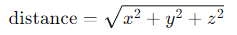
    Distance = sqrt((Position_X - &earth_position_x)**2 + (Position_Y - &earth_position_y)**2 + (Position_Z - &earth_position_z)**2);
    run;

    /* Calculate the minimum distance to Earth for each civilization */
    proc sql;
    create table civilization_min_distance as
    select Civilization, Distance as Min_Distance
    from civilization_distances
    order by Distance;
    quit;

    /* Calculate the probability of encountering civilizations based on distance */
    data probability_encounter;
    set civilization_min_distance;
    Probability = 1 / (1 + Min_Distance);
    run;

    /* Calculate the average probability for each distance band */
    proc sql;
    create table average_probability as
    select case
    when Min_Distance <= 1000 then 'Close'
    when Min_Distance > 1000 and Min_Distance <= 3000 then 'Medium'
    when Min_Distance > 3000 then 'Far'
    end as Distance_Band,
    avg(Probability) as Average_Probability
    from probability_encounter
    group by case
    when Min_Distance <= 1000 then 'Close'
    when Min_Distance > 1000 and Min_Distance <= 3000 then 'Medium'
    when Min_Distance > 3000 then 'Far'
    end;
    quit;

    /* Print the result */
    proc print data=average_probability;
    run;

    /* Select the closest civilization to Earth and its associated probability */
    proc sql;
    create table closest_civilization as
    select Civilization, Min_Distance, Probability
    from probability_encounter
    where Min_Distance = (select min(Min_Distance) from probability_encounter);
    quit;

    /* Print the result */
    proc print data=closest_civilization;
    run;


    /*Bayesian analysis for probability of encountering aliens in the past or future*/

    /* Set seed for reproducibility */
    %let num_iterations = 100;

    /* Create Bayesian analysis dataset */
    data bayesian_analysis;
    call streaminit(123);

    /* Define variables for posterior probabilities */
    array posterior_past[&num_iterations];
    array posterior_future[&num_iterations];

    do i = 1 to &num_iterations;
    /* Sample prior probabilities and likelihoods for past encounters */
    prior_past = rand("Uniform", 0.0001, 0.01); /* P(Past encounter) */
    likelihood_past_encounter = rand("Uniform", 0.001, 0.1); /* P(No contact | Past encounter) */
    likelihood_no_encounter_past = rand("Uniform", 0.8, 0.99); /* P(No contact | No encounter) */

    /* Calculate posterior probability for past encounter using Bayes' Theorem */
    numerator_past = prior_past * likelihood_past_encounter;
    denominator_past = numerator_past + (1 - prior_past) * likelihood_no_encounter_past;
    posterior_past[i] = numerator_past / denominator_past;

    /* Sample prior probabilities and likelihoods for future encounters */
    prior_future = rand("Uniform", 0.001, 0.05); /* P(Future encounter) */
    likelihood_future_encounter = rand("Uniform", 0.01, 0.1); /* P(No contact | Future encounter) */
    likelihood_no_encounter_future = rand("Uniform", 0.8, 0.99); /* P(No contact | No encounter) */

    /* Calculate posterior probability for future encounter using Bayes' Theorem */
    numerator_future = prior_future * likelihood_future_encounter;
    denominator_future = numerator_future + (1 - prior_future) * likelihood_no_encounter_future;
    posterior_future[i] = numerator_future / denominator_future;
    end;

    /* Output the results */
    do i = 1 to &num_iterations;
    posterior_past_value = posterior_past[i];
    posterior_future_value = posterior_future[i];
    output;
    end;
    keep posterior_past_value posterior_future_value;
    run;

    /* Summary statistics for the posterior probabilities */
    proc means data=bayesian_analysis mean std min max;
    var posterior_past_value posterior_future_value;
    run;

    /* Distribution histograms for the posterior probabilities */
    proc sgplot data=bayesian_analysis;
    histogram posterior_past_value / transparency=0.5 fillattrs=(color=blue) binwidth=0.00001;
    title "Distribution of Posterior Probabilities for Past Encounters";
    run;

    proc sgplot data=bayesian_analysis;
    histogram posterior_future_value / transparency=0.5 fillattrs=(color=green) binwidth=0.0001;
    title "Distribution of Posterior Probabilities for Future Encounters";
    run;

    With this code, we simulate both past and future alien encounters under a range of assumptions, enabling us to estimate the likelihood of each scenario using Bayesian reasoning. By the end of the process, we have distributions of probabilities for both past and future alien contact, which we’ll now analyze to gain further insights.

    Analyzing the Table and Graphical Output

    Table Output

    The table presents the summary statistics for the posterior probabilities, which represent the likelihood of both past and future alien encounters:

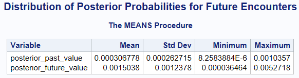
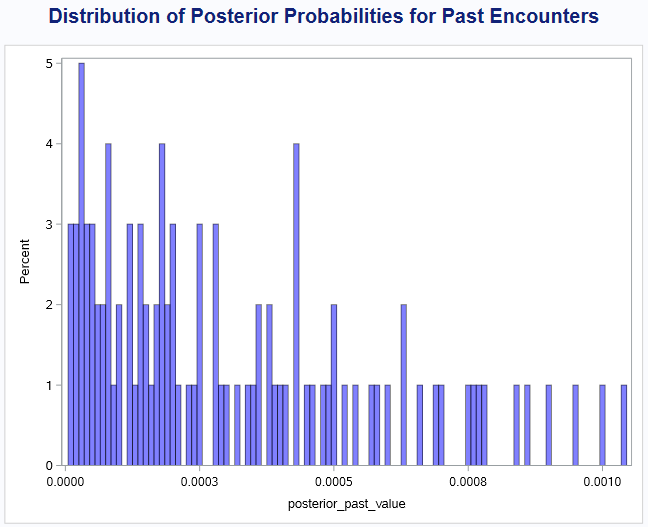
    posterior_past_value:

    • Mean: 0.000306778
    • Std Dev: 0.000262715
    • Minimum: 8.258388E-6
    • Maximum: 0.0010357

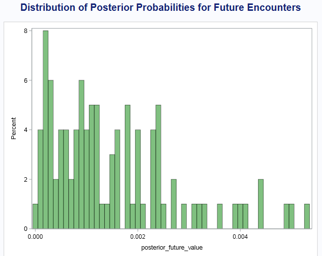
    posterior_future_value:

    • Mean: 0.0015038
    • Std Dev: 0.0012378
    • Minimum: 0.000036464
    • Maximum: 0.0052718

    Interpretation:

    • Past Encounters: The mean probability for past encounters is around 0.0003, or approximately 0.03%. In more intuitive terms, this translates to about a 1 in 3,260 chance that we’ve encountered aliens in the past.
    • Future Encounters: The mean probability for future encounters is higher, at around 0.0015, or 0.15%. This translates to about a 1 in 667 chance of encountering aliens in the future.

    The range of these values indicates that there is quite a bit of uncertainty, which makes sense given the limitations of the data and assumptions. The minimum value for past encounters is as low as 0.000008 (or 1 in 125,000), while the maximum value is closer to 0.001 (or 1 in 1,000). Future encounters range from 0.000036 (1 in 27,397) to 0.005 (or 1 in 190).

    Graphical Output

    1. Distribution of Posterior Probabilities for Past Encounters:
      The histogram shows a wide distribution, with most probabilities clustering around the lower end, below 0.0005. This suggests that the likelihood of past encounters is generally low across our simulations, but there are still a few instances where the probability was higher, approaching 0.001 (or 1 in 1,000).

    2. Distribution of Posterior Probabilities for Future Encounters:
    The distribution for future encounters is more spread out, with the highest probability occurrences clustered between 0.0005 and 0.002. This indicates that future encounters, while still unlikely, have a higher probability than past encounters. The shape of the distribution suggests that while the odds of contact are low, there is a non-trivial chance that future encounters could happen, depending on how certain assumptions play out.

    Key Takeaways and Probability Calculations

    Past Encounters:

    The mean posterior probability of a past encounter is approximately 0.0003. In terms of simple odds, this translates to a 1 in 3,260 chance that humanity has already encountered extraterrestrial life without realizing it. The wide distribution reflects uncertainty, with probabilities ranging from as low as 1 in 125,000 to as high as 1 in 1,000, depending on the assumptions we use for prior likelihoods and evidence.

    Future Encounters:

    The mean posterior probability for future encounters is 0.0015, which translates to a 1 in 667 chance that we will encounter alien life at some point in the future. While still unlikely, this higher probability compared to past encounters suggests a better (though still slim) chance of future contact. The distribution ranges from a 1 in 27,397 chance at the low end to a more optimistic 1 in 190 chance, reflecting the wide range of possible outcomes.

    Tying It All Together: What Does This Mean?

    The journey we’ve taken throughout this series has been a fascinating exploration of probability, uncertainty, and the grandest of questions: Are we alone in the universe? Using the Drake Equation as a framework, we’ve examined every step from the formation of habitable planets to the development of intelligent, communicative civilizations. But what does it all mean, and why did we take this approach?

    The Bigger Picture

    1. Why We Did This: Our goal was simple, yet profound: to rationally assess the likelihood of alien civilizations existing and, even more importantly, whether we have — or will ever — encounter them. There is a lot of speculation in popular culture about UFOs, sightings, and mysterious signals, but we wanted to approach this scientifically. By working through the Drake Equation, using Monte Carlo simulations, and applying Bayesian reasoning, we attempted to put some tangible numbers to an otherwise nebulous question.
    2. How We Did It: The methodology we used isn’t about definitive answers but rather about understanding the range of possibilities. Each step of the Drake Equation brings with it huge uncertainties — how many habitable planets exist, how many develop life, and how many civilizations are sending signals into the cosmos. To handle this uncertainty, we turned to Monte Carlo simulations, which allowed us to account for a broad range of outcomes and calculate distributions instead of single estimates. Bayesian analysis then helped us refine these probabilities based on current evidence — or the lack thereof — providing more nuanced predictions about alien contact.
    3. What the Results Mean: The numbers might seem small at first glance, but they are significant in their implications. The odds of past contact (about 1 in 3,260) are low, which isn’t surprising given the lack of definitive evidence. Yet, these odds are not zero, and that in itself is worth noting — there is a chance, however small, that we have already encountered extraterrestrial life without realizing it.
    4. The probability of future contact is a bit more optimistic: around 1 in 667. While still a long shot, this suggests that if we continue searching, there is a small but tangible chance we could detect or communicate with alien civilizations at some point in the future. The future is uncertain, but with advancing technology and an ever-expanding field of study in astrobiology and space exploration, the possibility remains.

    The Takeaway:

    This analysis leaves us with a sobering but hopeful conclusion. The universe is vast, and the distances between stars — let alone civilizations — are staggering. The very structure of the cosmos, combined with the timescales involved in the rise and fall of civilizations, suggests that encounters are improbable but not impossible.

    The true marvel here is not just in the numbers but in what they represent: the intersection of humanity’s curiosity and our capacity for rational, evidence-based exploration. We may be alone, or we may one day share a signal with another intelligent civilization. Either way, the work we’ve done to quantify the probabilities shows that the search itself is worthwhile. It reveals how much we still have to learn about the universe and our place in it.

    While the odds may not be in our favor, the possibility of a future encounter — however remote — gives us reason to keep looking to the stars. The universe remains full of mysteries, and our journey to solve them continues. Whether or not we ever make contact, the search itself pushes the boundaries of science, philosophy, and our collective imagination.

    This is where the work leaves us — not with concrete answers, but with profound questions that will continue to inspire curiosity, exploration, and wonder for generations to come. The search for extraterrestrial life is a search for understanding, not just of the cosmos, but of ourselves.

    If you missed the previous parts, start here.

    Unless otherwise noted, all images are by the author


    Are We Alone? was originally published in Towards Data Science on Medium, where people are continuing the conversation by highlighting and responding to this story.

    Originally appeared here:
    Are We Alone?

    Go Here to Read this Fast! Are We Alone?

  • Galactic Distances

    Galactic Distances

    James Gearheart

    How Far Are We from Alien Civilizations? (Part 4 of the Drake Equation Series)

    Recap:

    In our journey so far, we’ve walked through the Drake Equation to estimate how many civilizations might be “out there” in our galaxy. We’ve covered the stars, the planets that could support life, and how many might develop intelligent civilizations. In Part 3, we estimated how many of those civilizations are capable of communicating with us right now. Now, in Part 4, we’re facing the big question: How far away are they?

    The Milky Way is vast. We know there could be thousands of civilizations out there, but the galaxy is 100,000 light-years across — so even if they exist, could we ever hear from them? This article explores the mind-bending distances between us and these potential civilizations, and what that means for our search for extraterrestrial life.

    All images were developed by the author using Midjourney.

    How Big is Space? Putting the Vastness of the Milky Way into Perspective

    To put the vastness of space into perspective, let’s start by imagining the Milky Way galaxy, which spans about 100,000 light-years in diameter. Now, if we were to shrink the galaxy down to the size of Earth (with a diameter of about 12,742 kilometers), the relative size of Earth itself would become unimaginably small. In fact, Earth would be 742 billion times smaller in comparison — about the size of a single human red blood cell. This comparison illustrates just how immense our galaxy is and emphasizes the monumental challenge of exploring or communicating across such vast distances. Imagine the difficulty of trying to find a single red blood cell in a space the size of the Earth!

    Step 8: Estimating the Distance to the Nearest Alien Civilization

    The results from Part 3 suggested that there could be up to 2,363 alien civilizations communicating in our galaxy right now. But what does that mean in practical terms? If they’re out there, how close is the nearest one?

    Why This Step Matters

    Even if we know there are thousands of civilizations, distance is a huge hurdle. The farther away they are, the harder it is to detect their signals — or for them to detect ours. If we want to set realistic expectations for contacting these civilizations, we need to know how far away they are. And if they’re hundreds or even thousands of light-years away, it’s going to be tough to communicate in real time. Imagine sending a text, only to get a reply 2,000 years later!

    Our Approach

    We’re assuming that alien civilizations are randomly distributed throughout the Milky Way. This gives us a nice, even spread across the galaxy’s disk, which has a diameter of around 100,000 light-years and a thickness of 1,300 light-years.

    This approach keeps things simple while acknowledging that we’re making some big assumptions. For example, we’re not considering galactic zones that might be more “life-friendly,” and we’re ignoring the idea that some regions might be barren. But for our purposes, this model gives us a solid foundation for calculating the average distance to the nearest civilization.

    Code for Step 8: Calculating the Distance to the Nearest Alien Civilization

    ***********************************************************************
    *Calculate the distance to the closest civilization assuming that they
    *are randomly distributed across the galaxy
    ***********************************************************************

    data closest_civilization;
    /* Set seed for reproducibility */
    call streaminit(123);

    /* Define Parameters */
    %let num_civilizations = 2363;
    %let num_iterations = 100;

    %let galactic_radius = 50000;
    %let galactic_height = 1300;

    /* Initialize variables */
    length iteration 8 distance 8;
    array distances[&num_iterations]

    /* Calculate distances */
    do i = 1 to &num_iterations;
    /* Generate random coordinates for civilizations */
    do j = 1 to &num_civilizations;
    x = rand("Uniform", -&galactic_radius, &galactic_radius);
    y = rand("Uniform", -&galactic_radius, &galactic_radius);
    z = rand("Uniform", -&galactic_height, &galactic_height);

    /* Calculate distance from Earth */
    distance = sqrt(x**2 + y**2 + z**2)

    /* Update closest distance if applicable */
    if j = 1 then closest_distance = distance;
    else if distance < closest_distance then closest_distance = distance;
    end;

    /* Store closest distance */
    distances[i] = closest_distance;
    end;

    /* Output distances to dataset */
    do iteration = 1 to &num_iterations;
    distance = distances[iteration];
    output;
    end;

    /* Keep only the necessary variables */
    keep iteration distance;
    run;

    A Small Confession: I Cheated (and Gave Us Better Odds)

    Alright, time for a little confession: the Earth isn’t actually sitting in the middle of the galaxy, despite how I set up the code to calculate the distance to the nearest alien civilization. In reality, we’re about three-quarters of the way toward the edge of the Milky Way. If I had placed the Earth where it truly belongs, the average distance to alien civilizations on the far side of the galaxy would be much greater. But by “cheating” and moving us to the galactic center, I’ve inadvertently decreased the average distance to potential neighbors — and, in turn, increased our odds of contact. So yes, this biased approach works in our favor, but I’m sure you won’t mind if I made the cosmos feel a little cozier!

    Breaking Down the Code: Calculating the Distance to the Nearest Civilization

    This code is designed to simulate and calculate the distance from Earth to the nearest alien civilization, assuming that civilizations are randomly distributed throughout the Milky Way galaxy. Let’s walk through the key components and logic of the code.

    Overview of the Key Variables

    • num_civilizations: This is set to 2,363, which is the number of civilizations we estimated in Part 3 to be communicating at the same time as us. This parameter is the foundation of our calculation, as we want to figure out how far the closest of these civilizations might be from us.
    • galactic_radius and galactic_height: These parameters define the size of the Milky Way. The galaxy is modeled as a disk, 100,000 light-years in diameter (which gives us a radius of 50,000 light-years) and 1,300 light-years thick.
    • num_iterations: The code will run 100 iterations of the simulation, meaning it will randomly distribute the civilizations and recalculate the distance multiple times to get a range of possible distances to the nearest civilization.

    Setting Up the Simulation

    • Random Seeding (call streaminit(123)): This is for reproducibility. By setting a seed value (123), we ensure that every time we run this code, we get the same random values, making the results consistent across multiple runs.
    • Random Galactic Coordinates: Each alien civilization is randomly placed in the galaxy by generating random (x, y, z) coordinates, with x and y representing the positions within the galaxy’s disk (radius), and z representing the position relative to the height of the galaxy (its thickness). The rand(“Uniform”,…) function generates random values within the specified ranges:
    • The x and y coordinates are picked from a range of -50,000 to +50,000 light-years to cover the full width of the galaxy.
    • The z coordinate is picked from a range of -1,300 to +1,300 light-years to represent the galaxy’s thickness.

    Calculating Distance from Earth

    The next section of the code calculates the distance from Earth (located at the origin, [0, 0, 0]) to each randomly positioned alien civilization using the 3D distance formula:

    This formula calculates the straight-line distance from Earth to each civilization based on its random galactic coordinates.

    Finding the Closest Civilization

    Now that we have the distances, the code checks which one is the closest:

    • First Civilization: On the first iteration (when j = 1), the first calculated distance is stored as the closest distance, because at this point, there’s nothing to compare it to.
    • Subsequent Civilizations: For each additional civilization, the code compares its distance to the previously stored closest distance. If the new distance is smaller, it updates the value of closest_distance.

    Storing and Outputting the Results

    • Storing the Closest Distance: The closest distance found in each iteration is stored in the array distances[]. This allows us to keep track of the closest civilization for each simulation run.
    • Output the Distances: The do loop at the end outputs the distance data for each iteration, so we can analyze the distribution of these results. It’s essentially producing a dataset of distances for all 100 simulation runs.

    What This Code Is Doing

    This simulation is creating random galactic coordinates for 2,363 civilizations in each iteration, calculating the distance to Earth for each one, and identifying the closest civilization. It repeats this process 100 times, giving us a range of possible distances to the nearest alien civilization based on the assumptions we’ve made.

    Why This Matters

    This is a crucial step in understanding the practical challenge of contacting extraterrestrial civilizations. Even if there are thousands of civilizations, the closest one could still be far beyond our reach. By simulating random distributions, we get an idea of the minimum distance we’d need to cover to contact another civilization — which sets realistic expectations for the search for extraterrestrial life.

    Output and Explanation: Distance to the Nearest Civilization

    Now for the results! After running the simulation, we get the following estimates for the distance to the nearest alien civilization, based on our earlier calculations:

    • Minimum Number of Civilizations (1): 39,594 light-years away.
    • Mean Number of Civilizations (2,363): 1,283 light-years away.
    • Maximum Number of Civilizations (500,299): 214 light-years away.

    What Does This Tell Us?

    • The Closest Possible Civilization: If we take the optimistic scenario where there are half a million alien civilizations, the nearest one would be just over 200 light-years away. This is within a range that we could theoretically detect with current technology, but it’s still a long shot.
    • The Most Likely Scenario: With our mean estimate of 2,363 civilizations, the nearest one is likely around 1,283 light-years away. For perspective, that means a signal we send today wouldn’t reach them for over a millennium — and we wouldn’t get a reply until another millennium had passed!
    • The Worst-Case Scenario: If there’s only one other civilization out there, it could be nearly 40,000 light-years away, making contact almost impossible.

    Why This Matters

    Even with the exciting possibility of thousands of alien civilizations, the sheer distances between us are daunting. On average, we’re looking at over 1,000 light-years to the nearest civilization, which means that communication is a long shot — at least with our current technology. But that doesn’t mean the search is hopeless. It just means we need to adjust our expectations and think about more indirect ways to detect signs of intelligent life.

    Step 9: Traveling the Cosmic Distances — The Role of Relativity

    So, let’s say we somehow knew where an alien civilization was located. How long would it take to reach them? This is where things get even more mind-bending — because when you’re talking about interstellar distances, you have to think about Einstein’s theory of special relativity.

    Understanding the Lorentz Factor

    At the heart of special relativity is the Lorentz Factor. This concept explains how time and space behave as objects approach the speed of light, and it’s key to understanding how interstellar travel might work.

    Here’s the formula:

    Where:

    • v is the velocity of the spacecraft (or any object moving through space).
    • c is the speed of light.

    What this equation tells us is that as an object’s velocity v gets closer to the speed of light c, the Lorentz Factor γ grows larger. This leads to two key effects:

    • Time Dilation: Time slows down for the travelers on the spacecraft. If you’re zooming through space at close to light speed, you experience less time than those on Earth. So, a trip that takes thousands of years from Earth’s perspective might only feel like a few years to the travelers.
    • Length Contraction: The distance to your destination appears shorter. As you approach the speed of light, distances seem to shrink for the people on the spacecraft.

    Now, let’s apply this to our scenario.

    Code for Step 9: Calculating Travel Time and the Lorentz Factor

    ***************************************************************;
    *How long is the travel time given different distances and ;
    *different "% of speed of light" ;
    ***************************************************************;

    /* Constants */
    data _null_;
    speed_of_light = 299792.458; /* km/s */
    distance_ly = 100; /* Light years */
    distance_km = distance_ly * 9.461 * 10**12; /* Conversion to kilometers */
    travel_distance = distance_km;
    travel_time = travel_distance / (0.9 * speed_of_light); /* Convert to seconds and reduce top speed of ship
    to % of the speed of light*/

    put "Travel Distance (km): " distance_km;
    put "Travel Time (seconds): " travel_time;

    velocity = travel_distance / travel_time;

    lorentz_factor = 1 / sqrt(1 - (velocity**2 / (speed_of_light**2)));
    proper_time_sp = travel_time / lorentz_factor; /* unit of time experienced on spaceship */
    time_dilation_sp = proper_time_sp / (365.25 * 24 * 60 * 60); /* converting to years */
    time_earth = travel_time / (365.25 * 24 * 60 * 60); /* converting to years */

    put "Velocity: " velocity;
    put "Lorentz Factor: " lorentz_factor;
    put "Proper Time (Spaceship): " proper_time_sp " seconds";
    put "Time Dilation (Spaceship): " time_dilation_sp " years";
    put "Time (Earth): " time_earth " years";
    run;

    Breaking Down the Code: Calculating Travel Time and Time Dilation

    This code is designed to calculate how long it would take a spacecraft to travel between Earth and the nearest alien civilization at a fraction of the speed of light. It also calculates the time dilation experienced by the travelers due to Einstein’s theory of special relativity. Let’s break it down step by step to understand how these calculations work and why they’re important.

    Constants and Basic Calculations

    1. Speed of Light:
    • The speed of light, denoted as speed_of_light, is a well-known constant set at 299,792.458 km/s. This is the maximum speed limit for any object according to the laws of physics, and it forms the basis for our travel calculations.

    2. Distance to the Closest Civilization:

    • We set the distance to the nearest civilization (distance_ly) at 1,283 light years (a placeholder value). This number represents the distance we estimated in earlier steps, based on the distribution of civilizations.

    3. Convert Distance to Kilometers:

    • Since the speed of light is in km/s, we need to convert the distance from light years to kilometers:

    A light year is approximately 9.461 trillion kilometers, so this conversion gives us the total distance in kilometers, which is crucial for the travel time calculation.

    Calculating Travel Time

    1. Fraction of the Speed of Light:
    • The example below calculates the travel time based on a ship traveling at 1% of the speed of light. The formula used for travel time is:

    This formula converts the total distance to the time it would take the spacecraft to cover that distance at 1% of the speed of light. The output is in seconds, which gives us the most precise calculation.

    2. Print Travel Distance and Time:

    • The program outputs the total distance (in kilometers) and travel time (in seconds) to give us a sense of the scale we’re dealing with.

    Special Relativity and Time Dilation

    In this part of the code, we’re revisiting Einstein’s theory of special relativity, focusing on time dilation as it relates to interstellar travel. We previously discussed the Lorentz Factor, which plays a crucial role in determining how time slows down for objects moving at speeds close to the speed of light.

    But why are we using the Lorentz Factor here?

    Why the Lorentz Factor Matters

    In the context of interstellar travel, as a spacecraft’s velocity approaches the speed of light, the Lorentz Factor increases dramatically. This has two significant effects:

    1. Time Dilation: The time experienced by the crew aboard the spacecraft would be much shorter than the time experienced by observers on Earth. In essence, while the journey might take centuries or millennia from Earth’s perspective, only a few years could pass for the crew.
    2. Perception of Distance: The faster the spacecraft travels, the shorter the distance appears to those on board. This contraction of space, caused by the Lorentz Factor, means that the crew would perceive the journey as much shorter than the actual distance across space.

    Impact on Travel Time

    By incorporating the Lorentz Factor, the code allows us to calculate two important results:

    • Proper Time on the Spaceship: The amount of time the crew would experience while traveling across vast distances. Thanks to time dilation, this will be significantly shorter than the time that passes on Earth.
    • Time on Earth: The total time it would take from an Earth-bound perspective to reach a distant alien civilization. Even at high speeds, the journey could span centuries or longer.

    This is why the Lorentz Factor is critical: it lets us understand how time and space behave at relativistic speeds, giving us a glimpse into the effects that would make long-distance space travel more manageable for the travelers, though still incredibly challenging from an Earth-bound perspective.

    Final Output

    The code outputs several key insights:

    • Velocity: The spacecraft’s speed as it approaches a percentage of the speed of light.
    • Lorentz Factor: How much time dilation is occurring due to the spacecraft’s speed.
    • Proper Time: The journey’s duration as experienced by the crew.
    • Time on Earth: How much time would pass for those remaining on Earth while the journey is undertaken.

    Why This Matters

    This section highlights the staggering complexity of interstellar travel. Even though the crew would experience a much shorter journey thanks to time dilation, the distance between Earth and potential alien civilizations remains immense. The Lorentz Factor illustrates how the laws of physics influence not only the speed of travel but also the perception of time and distance. While time dilation offers a potential advantage for long-distance voyages, the journey to a distant civilization remains a monumental task, requiring technology far beyond what we currently possess.

    Output and Explanation: Traveling the Cosmic Distances

    Now, we’ve come to the moment of truth — understanding just how long it would take to reach the nearest alien civilization given the vast distances of space and different travel speeds.

    Travel Time to the Nearest Civilization

    We’ve assumed that the nearest alien civilization is 1,283 light-years away, based on our earlier estimates. Here’s where things get fascinating. The travel time varies dramatically depending on how fast the spacecraft is traveling relative to the speed of light. Let’s explore these numbers:

    • At 1% the Speed of Light: The journey would take a staggering 128,303 years from Earth’s perspective. To put that into context, Homo sapiens would have been living alongside Neanderthals and saber-toothed cats during the Ice Age if this trip had started that long ago!
    • At 10% the Speed of Light: The trip would still take 12,830 years from Earth’s point of view — that’s around the time of the end of the Ice Age, when humans began migrating and megafauna like mammoths were going extinct.
    • At 50% the Speed of Light: We start seeing more manageable numbers. The journey would take 2,566 years from Earth’s perspective, which means that when the spacecraft left, humanity would have been in the time of Jesus, ancient Greece, Egypt, and the rise of Buddhism.
    • At 90% the Speed of Light: Now we’re getting somewhere! The trip would take 1,425 years from Earth’s perspective. Think about that: when the travelers set off, the Byzantine Empire was at its height, the Tang Dynasty ruled China, and the Maya civilization was flourishing.
    • At 99% the Speed of Light: The journey now takes just 1,295 years from Earth’s perspective. To put that in context, Vikings were sailing the seas, and Anglo-Saxon kingdoms were being established in what is now England.

    But there’s more. These figures show time from Earth’s point of view, but for the astronauts on the spacecraft, time dilation caused by traveling at near-light speeds means they’ll experience much less time passing.

    Why Time Dilation is Crucial

    As the spacecraft approaches the speed of light, time dilation becomes an extraordinary advantage for the travelers:

    • At 50% the Speed of Light, while 2,566 years would pass on Earth, the crew would only experience 2,222 years.
    • At 90% the Speed of Light, while 1,425 years would pass on Earth, the crew would only feel 621 years passing. That’s enough for the journey to span multiple human generations, but it makes the idea of interstellar travel more feasible — at least for those aboard the spacecraft.
    • At 99% the Speed of Light, this becomes even more dramatic. While the journey would take 1,295 years from Earth’s perspective, the crew would only experience 183 years.

    The effect of time dilation means that, for the crew, the journey might feel much shorter, even though centuries or millennia would pass back home on Earth. This is why special relativity is so important in understanding the feasibility of interstellar travel. It’s not just about how long the trip takes — it’s about how time itself is experienced differently depending on the speed you’re traveling at.

    Why This Matters

    This simulation demonstrates that interstellar travel may be possible, but it’s not without enormous challenges. Time dilation offers an advantage to the crew on the spacecraft, but the vast distances mean that even at near-light speeds, the journey could take centuries or more from Earth’s perspective.

    The interplay of distance, speed, and time reveals just how difficult — but also fascinating — it would be to travel across the cosmos. While the travelers may experience only a few hundred years, their destination could still be over a millennium away from Earth’s perspective. This provides a striking reminder of the immense scales involved when contemplating the possibility of contacting alien civilizations.

    Transition to Part 5: The Final Challenge — Have We Ever Encountered Alien Life?

    Now that we’ve tackled the vast distances between civilizations, we face our final challenge: Could we have already encountered alien life and not known it? Or more excitingly, what are the odds we will encounter alien life in the future? In Part 5, we’ll dive into these probabilities, exploring past and future encounters, and what they mean for the future of humanity and the search for extraterrestrial intelligence.

    Stay tuned for the grand finale of the Drake Equation series!

    Next in the series: Are We Alone?: The Real Odds of Encountering Alien Life? (Part 5 of the Drake Equation Series). Or, if you missed the previous part, go back here.

    Unless otherwise noted, all images are by the author


    Galactic Distances was originally published in Towards Data Science on Medium, where people are continuing the conversation by highlighting and responding to this story.

    Originally appeared here:
    Galactic Distances

    Go Here to Read this Fast! Galactic Distances

  • Communicating with the Cosmos

    Communicating with the Cosmos

    James Gearheart

    Estimating Alien Civilizations (Part 3 of the Drake Equation Series)

    Welcome back! In Part 1, we began by estimating how many stars in our galaxy could have planets. In Part 2, we narrowed it down further to estimate how many planets could support life and how many of those might evolve intelligent civilizations. Now, in Part 3, we’ll take these estimates one step further, estimating how many intelligent civilizations have developed communication technology.

    But here’s the big question: How many of those civilizations might be communicating with us right now?

    A Quick Recap of the Drake Equation

    Before we dive in, let’s quickly review the steps of the Drake Equation we’ve covered so far:

    Drake Equation:

    1. R = How many stars are in the galaxy?
    2. f_p = How many of those stars have planets?
    3. n_e = How many planets are in the habitable zone?
    4. f_l = How many of those planets develop life?
    5. f_i = How many planets with life evolve intelligent civilizations?

    Now, we’re focusing on Step 6: How many civilizations develop technology that could communicate across interstellar distances?

    All images were developed by the author using Midjourney.

    Step 6: Fraction of Civilizations that Develop Communication Technology (f_c)

    We’ve established that intelligent life may exist, but here’s the kicker — just because a civilization is smart doesn’t mean they have the technology (or the desire) to communicate across space. In fact, many advanced civilizations could be using technologies that are completely undetectable to us.

    For our purposes, we’re defining communication ability as the development of technology that allows civilizations to send signals detectable by our current instruments — things like radio waves or lasers. Sure, some civilizations might use more exotic methods (gravity waves, quantum entanglement, etc.), but for now, we’re sticking to what we can realistically detect.

    Why We Chose This Range

    We estimate that between 10% to 20% of intelligent civilizations develop communication technology, with an average of 15%. The reasoning? Developing communication technology involves several “hard steps,” and not every civilization will take the same path. Let’s break it down:

    • Surviving Extinction-Level Events: Just like Earth has experienced mass extinctions, other civilizations may face natural disasters or wars. A civilization can’t communicate if it doesn’t survive.
    • Developing Technology: Even if a civilization becomes intelligent, there’s no guarantee they’ll prioritize communication tech. They might stay local or even evolve beyond detectable technology.
    • Communicating in a Detectable Form: Even if they develop technology, they have to communicate in ways we can detect — like radio waves. If they use more advanced forms, we wouldn’t be able to hear them.

    Let’s see how this plays out in the simulation. First, we’ll run some SAS code to generate 100,000 values based on the distribution we’ve chosen for this step.

    Code for Step 6: Calculating the Fraction of Civilizations with Communication Technology

    /*Percent of Intelligent Life with Communication Ability*/

    data perc_comm_ability(keep=perc_comm_ability);
    do i = 1 to 100000;
    do while (1);
    perc_comm_ability = rand("normal", 0.15, 0.015);
    /* Check if the value is within the desired range */
    if perc_comm_ability >= 0.1 and perc_comm_ability <= 0.2 then leave;
    end;
    output;
    end;
    drop i;

    format perc_comm_ability percent7.4;
    run;

    Output and Explanation for Step 6: Communication-Developing Civilizations

    After running the simulation, we established that the average percentage of civilizations that develop communication technology is around 15%, with values ranging from 10% to 20%.

    Breaking Down the Results

    • 1 in 6 civilizations: Roughly 1 out of every 6 intelligent civilizations reaches the point where they develop the technology to communicate across space.
    • Distribution: The results mostly cluster around 15%, with some variation between 10% and 20%. This gives us a solid foundation for moving forward to calculate the total number of communicative civilizations.

    Why These Results Matter

    This step in the Drake Equation is critical. Without the ability to communicate, even if intelligent civilizations exist, we’d never know. The results show that while not every intelligent civilization develops communication technology, a decent fraction likely does. This boosts our chances of making contact.

    Taking a Slight Detour from the Traditional Drake Equation

    At this point, we’re going to take a small divergence from the traditional Drake Equation before moving forward to calculate the total number of civilizations. Instead of directly incorporating the length of time that civilizations stay communicative (L) into the equation at this step, we’re first going to calculate a raw estimate for the total number of civilizations that ever developed communication abilities.

    Why This Divergence?

    The reason for this slight adjustment is that we want to separate two important concepts:

    1. The Total Number of Civilizations That Ever Existed: This gives us a raw number of civilizations in the galaxy that reached the point of developing communication abilities. This estimate doesn’t yet account for the fact that civilizations may rise and fall over time.
    2. The Overlap of Their Lifespan with Ours: This is where the concept of communicative lifespan comes in. After estimating the raw number of civilizations, we will later adjust that estimate to figure out how many of these civilizations might be active and communicative at the same time as our own.

    By taking this detour, we get a clearer picture of the total potential for communicative civilizations and then zoom in on how many might overlap with our present era. This approach allows us to get a comprehensive understanding of the total number of civilizations that ever existed before accounting for the communication lifetimes.

    Now, with that explanation in place, let’s move on to the next calculation: multiplying the distributions together to estimate how many civilizations have developed communication abilities across the history of the Milky Way.

    Multiplying the Distributions Together

    Now that we’ve calculated the fraction of intelligent civilizations that develop communication technology, it’s time to multiply all the distributions together. This will give us an estimate for the total number of alien civilizations that ever developed communication technology in the Milky Way.

    This step involves multiplying the results from each part of the Drake Equation so far:

    • Total number of stars
    • Fraction of stars with planets
    • Fraction of planets in the habitable zone
    • Fraction of planets where life develops
    • Fraction of planets where intelligent life emerges
    • Fraction of intelligent civilizations that develop communication technology

    Output and Explanation for the Total Number of Communicative Civilizations

    After running the final calculation, we estimate that there are 96,828 alien civilizations that have developed communication technology throughout the history of the Milky Way.

    What Do These Results Mean?

    • A Vast Number: The total number of 96,828 civilizations is incredibly large, but it includes all civilizations that have ever existed and developed communication technology. This number covers billions of years of galactic history.
    • Galactic Potential: While the sheer size of this number is impressive, the real question is how many of these civilizations are broadcasting signals right now.

    Step 7: How Long Do Civilizations Stay in the “Communication Phase”? (L)

    We’ve estimated how many civilizations could develop communication abilities, but now we ask: how long do they stay in this phase? Civilizations might rise and fall, and their ability to send detectable signals could be brief. For instance, humanity has only been sending signals into space for about 100 years, and it’s uncertain how long we’ll continue. Natural disasters, resource depletion, or even self-destruction could end any civilization’s communicative phase.

    Why We Diverge from the Traditional Drake Equation

    In the original Drake Equation, the lifespan of civilizations is calculated early on. However, in our approach, we first calculate the raw estimate of all civilizations that have developed communication abilities. Then, we bring in the concept of their lifespan to see how many might overlap with our own civilization. This helps us focus on the civilizations that are still active right now.

    Galactic Communication Lifespan

    The length of time a civilization remains communicative depends on several factors:

    • Surviving extinction-level events: Natural or self-induced disasters like asteroid impacts or nuclear wars can easily cut short a civilization’s ability to communicate.
    • Technological development: A civilization must develop the means to transmit signals across space, which could take thousands of years.
    • Maintaining communication: Even if they develop communication technologies, civilizations might abandon them or switch to undetectable methods as they evolve.

    Humanity’s Communicative Age: A Tiny Window

    For perspective, while Homo sapiens have existed for 200,000 years, we’ve only been capable of sending signals for just over 100 years. That’s a minuscule fraction of our existence. More intentional attempts to communicate, like the Arecibo message in 1974, only began 50 years ago. This suggests the communicative phase for any civilization could be very short.

    Modeling Civilization Lifespan

    In our analysis, the L factor represents the length of time a civilization remains communicative, sending out signals that could be detected by others. We modeled this with a distribution designed to ramp up quickly from short-lived civilizations (e.g., a few hundred or thousand years) to longer-lasting ones.

    Why We Chose This Range

    We intentionally set L to start low — around 100 years — but ramp up after that. The reasoning is simple: if a civilization can survive the first 100 to 500 years of its technological development, it’s more likely to last much longer, potentially even thousands of years.

    Running the Simulation

    With these assumptions, we run the simulation to estimate how long civilizations remain communicative, accounting for both short-lived and long-lasting civilizations.

    /*Years of Communicative Abilities*/

    data lifetime_comm_civ(keep=lifetime_comm_civ);
    skewness = -6; /* Control the left skewness */
    sigma = (log((1 + (skewness ** 2)) ** 0.5)) / skewness; /* Calculate sigma for Lognormal distribution */

    /* Generate random values from a left-skewed Lognormal distribution */
    do i = 1 to 100000;
    u = rand("uniform"); /* Uniform random variable */
    lifetime_comm_civ = 100 + (1000000 - 100) * exp(sigma * rand("lognormal", 0, 1));
    output;
    end;

    run;

    Output and Explanation for Step 7: Civilization Lifespan

    After running our simulation for the L factor (the length of time civilizations remain communicative), the results show a diverse range of lifespans. Let’s break down the key points:

    Key Statistics

    • Mean lifespan: 680,330 years.
    • Median lifespan: 739,262 years.
    • Range: From a minimum of 100 years to a maximum of 996,193 years.

    Distribution Insights

    • Average and Median: The average lifespan of a communicative civilization is 680,330 years, but notice that the median is a bit higher, at 739,262 years. This indicates that while some civilizations do last shorter periods, the distribution tends to favor civilizations that last quite long — hundreds of thousands of years.
    • Min and Max: The minimum lifespan, at 100 years, represents civilizations that quickly exit the communicative phase. The 1% quantile (46,758 years) shows that even the civilizations in the bottom tier last a significant amount of time on cosmic scales. At the upper end, a small number of civilizations could persist for almost 1 million years.
    • Skewness and Ramp Up: As intended, the distribution is left-skewed, meaning most civilizations reach the 10,000-year mark quickly and then extend much further into long timeframes. This is particularly evident in the sharp increase between the 1% quantile (46,758 years) and the median (739,262 years).

    What Does This Mean?

    The distribution suggests that, once civilizations make it past early hurdles (e.g., 10,000–50,000 years), many of them survive for extended periods, increasing the likelihood of sustained communication. The fact that the average civilization could last over 600,000 years is good news for our search — if civilizations manage to survive past their infancy, there’s a strong chance they will remain communicative for a substantial amount of time, making it more likely that their signals overlap with our own civilization’s brief window of communication.

    Transitioning from Communication Lifespan to Current Alien Civilizations

    Now that we’ve estimated the lifespan of civilizations in their communicative phase, the next key question is: how many of those civilizations exist right now? This is where our divergence from the traditional Drake Equation comes into play. Rather than just asking how many civilizations have ever existed, we need to factor in the overlap between their communicative phase and our own. After all, it’s only civilizations that are sending out signals during our brief window of existence that we have any chance of detecting.

    With the lifespan of civilizations ranging from just a few hundred to potentially millions of years, we have to account for the possibility that many civilizations may have risen and fallen long before we came along — or might emerge long after we’re gone.

    Why Timing Matters: Galactic Timeframes The universe has been around for about 14 billion years, and the Milky Way galaxy alone is about 13.6 billion years old. Civilizations could have emerged billions of years ago and already vanished. This is why time overlap is so crucial. Even if a planet developed intelligent life, that civilization could have flourished and disappeared without ever intersecting with our own existence.

    So, how do we calculate the odds of civilizations existing at the same time as us?

    We estimate the age of our own civilization as around 10,000 years. That’s 5,000 years older than the Sumerians, and it assumes that our civilization and our technological advancement continues long into the future without interruptions like self-destruction or environmental collapse.

    To find the civilizations that are overlapping with us, we take the total number of communicative civilizations and calculate the proportion that exists during our specific timeframe.

    Code to Calculate the Probability of Overlapping Civilizations

    Using the lifespan estimates of civilizations in their communicative phase, we multiply the time overlap by the total number of potential civilizations. This calculation helps us figure out how many alien civilizations might be communicative at the same time as our own.

    /* Define the timeframe of our civilization */
    %let civilization_timeframe = 10000; /* in years */

    /* Calculate the estimated number of alien civilizations that exist at the same time */
    data time;
    set drake;
    civilizations_same_time = min(&civilization_timeframe, lifetime_comm_civ) * total_civ / lifetime_comm_civ;
    run;
    /*Taking the min value in the numerator ensures that we consider only the overlapping period between
    our civilization and the alien civilizations*/

    What’s Happening Here?

    Defining our civilization’s timeframe:

    • In this code, we’re setting the duration of our civilization’s “communicative phase” to 10,000 years. This represents the estimated length of time that human civilization might be capable of sending and receiving signals across space. We assume that humanity is 5,000 years older than the Sumerians, and this figure includes our own technology lifespan.

    Calculating the overlapping civilizations:

    • total_civ represents the total number of civilizations estimated to exist in the galaxy (the number we calculated by multiplying all the terms of the Drake Equation).
    • lifetime_comm_civ is the lifespan of a civilization’s communicative phase.

    We use the min() function to find the shorter of two values.

    • Our civilization’s communicative phase (civilization_timeframe), or
    • The alien civilization’s communicative phase (lifetime_comm_civ).

    This ensures that we’re only considering civilizations whose communicative lifespan overlaps with ours.

    • Why divide by lifetime_comm_civ? Dividing by the communicative lifespan helps standardize the result, ensuring that we only count civilizations that have communication windows overlapping with our own.

    The Importance of Overlap

    Civilizations can rise and fall over the galaxy’s 14-billion-year history. Even if 96,000 civilizations exist, many might have been active millions of years ago and are no longer broadcasting signals. We only care about civilizations that exist at the same time as us. The code ensures that we estimate this overlap accurately by focusing on how long both civilizations remain capable of communicating. Only overlapping lifespans count toward the final number of communicative civilizations.

    The Moment We’ve Been Building Toward: How Many Civilizations Are Out There Right Now?

    After running the simulations, considering the number of stars, habitable planets, life-bearing planets, and the development of intelligent civilizations with the ability to communicate, we’ve arrived at a pivotal question: how many of these civilizations are out there right now, at this very moment?

    Drumroll, please…

    Based on our calculations, we estimate that, on average, there are 2,363 civilizations currently existing in our galaxy with the ability to communicate. That’s right — 2,363 civilizations, each potentially broadcasting their presence across the cosmos, right at this moment!

    To put it in perspective: this isn’t just a number. This represents thousands of intelligent civilizations that could be spread across the Milky Way, possibly wondering about us, just as we are about them. The thought that there might be thousands of civilizations, some perhaps far more advanced than us, waiting to be discovered is both mind-boggling and thrilling.

    But before we get ahead of ourselves, there’s still one big question left to answer…

    How Close Are They?

    Having an estimated number of communicative civilizations is only half the battle. The next challenge is determining where they are. Could the closest alien civilization be within our technological reach? Or are they so far away that even if they’re transmitting signals, we might never know? In the next part, we’ll dive into the incredible distances between these civilizations and calculate just how far we’d have to go to find our cosmic neighbors.

    Stay tuned for Part 4 as we explore the galactic distances that separate us from potentially life-changing contact!

    Next in the series: Galactic Distances: How Far Away Are Alien Civilizations? (Part 4 of the Drake Equation Series). Or, if you missed the previous part, go back here.

    Unless otherwise noted, all images are by the author


    Communicating with the Cosmos was originally published in Towards Data Science on Medium, where people are continuing the conversation by highlighting and responding to this story.

    Originally appeared here:
    Communicating with the Cosmos

    Go Here to Read this Fast! Communicating with the Cosmos

  • From Stars to Life

    From Stars to Life

    James Gearheart

    A Data-Driven Journey (Part 2 of the Drake Equation Series)

    In Part 1, we explored how many stars in our galaxy might have planets, and we used data to estimate the total number of stars with planets in the Milky Way. Now that we’ve tackled the stars, let’s take a closer look at the planets themselves. In Part 2, we’ll dive into how many of those planets could actually support life, how often life emerges, and how likely it is that life evolves into intelligent civilizations — like us.

    As we continue through the Drake Equation, things get a bit more speculative. But don’t worry, we’ll use data science, Monte Carlo simulations, and reasonable assumptions based on current research to keep things grounded.

    All images developed by the author using Midjourney.

    Quick Reminder: The Drake Equation

    Just to refresh your memory, the Drake Equation breaks down the steps to estimate the number of active, communicative alien civilizations. Here’s a look at the full equation again:

    Step 3: How Many Planets Are in the Habitable Zone? (n_e)

    Not all planets are created equal — some are too hot, some too cold, and a few are just right. These “Goldilocks” planets sit in the habitable zone around their star, where conditions are just right for liquid water to exist. Liquid water is crucial because it’s a key ingredient for life as we know it. Planets that are too close to their star may be too hot, boiling away any water and potentially getting bombarded with harmful radiation. On the flip side, planets that are too far away are likely cold, icy worlds where liquid water can’t exist.

    So, how many of these habitable-zone planets are out there?

    Why We Chose This Range

    Recent discoveries of exoplanet systems like TRAPPIST-1 suggest that several planets might be in the habitable zone of their star. Based on this and current research, we estimate that 1% to 20% of planets in any given system fall into this category, with an average around 10%. We chose a normal distribution for this step, assuming that habitable planets are more common in the middle of this range, but with room for uncertainty on either side.

    Before we dive into the results, let’s set the stage with some SAS code to calculate this estimate.

    /*Percent of Habitable Planets*/

    data habitable_planets(keep=habitable_planets);
    do i = 1 to 100000;
    do while (1);
    habitable_planets = rand("normal", 0.10, 0.025);
    /* Check if the value is within the desired range */
    if habitable_planets >= 0.01 and habitable_planets <= 0.2 then leave;
    end;
    output;
    end;
    drop i;

    format habitable_planets percent7.4;
    run;

    Output and Explanation for Step 3: Habitable Planets

    After running the simulation, the average percentage of planets in the habitable zone came out to be 10%, with values ranging between 1% and 20%.

    What Do These Results Mean?

    • Balanced Estimate: The majority of the results clustered around the 10% mark, meaning that, on average, 1 out of every 10 planets could be in the habitable zone of their star.
    • Room for Uncertainty: The range we chose acknowledges the possibility that some planetary systems might have none, while others could have multiple planets in the habitable zone, giving us flexibility in our estimates.

    Step 4: How Often Does Life Actually Develop? (f_l)

    Not all planets are created equal — some are too hot, some too cold, and a few are just right. These “Goldilocks” planets sit in the habitable zone around their star, where conditions are perfect for liquid water to exist. Liquid water is crucial because, as far as we know, it’s a key ingredient for life. However, we have to acknowledge that our sample size for life-bearing environments is extremely small — in fact, it’s just one: Earth.

    Our understanding of the conditions needed for life is entirely based on carbon-based life forms like the ones we find here. Planets that are too close to their star may be too hot, evaporating away any potential water and suffering from high levels of radiation. On the other hand, planets too far from their star are likely cold, icy worlds where liquid water can’t survive. While we know life thrives in a narrow range of conditions here on Earth, this is guesswork beyond our planet.

    For this analysis, we’re focusing only on the kind of life we know — carbon-based organisms that need water, not more exotic ideas like silicon-based life forms or inter-dimensional beings.

    Why We Chose This Range

    We estimate that life develops on 1% to 25% of habitable planets, with an average around 17%. To reflect the possibility that life might have a higher chance of appearing when the conditions are just right, we use a left-skewed distribution. This means that while life may not always appear, when it does, it has a good shot of thriving.

    Let’s jump into the code and see what the simulation tells us.

    /*Percent of Habitable Planets where Life Develops*/

    data perc_life_develop;
    mean_pct = 0.15; /* Mean percentage */
    skewness = -6; /* Control the left skewness */
    sigma = (log((1 + (skewness ** 2)) ** 0.5)) / skewness; /* Calculate sigma for Lognormal distribution */

    /* Generate random values from a left-skewed Lognormal distribution */
    do i = 1 to 100000;
    u = rand("uniform"); /* Uniform random variable */
    perc_life_develop = 0.001 + (0.25 - 0.001) * exp(sigma * rand("lognormal", 0, 1));
    output;
    end;

    format perc_life_develop percent7.4;
    run;

    Output and Explanation for Step 4: Life-Developing Planets

    After running our simulation, we found that the average percentage of habitable planets where life develops is 17.08%, with values spread between 1% and 25%. Let’s break down what this means for our overall analysis.

    Breaking Down the Results

    • “Life Finds a Way”: As Spielberg’s famous quote suggests, our simulation reflects that, when conditions are favorable, life is likely to emerge. With an average of 17.08%, this suggests that nearly 1 in 6 habitable planets could develop life. This is an optimistic outcome, given that the appearance of life requires a multitude of factors aligning perfectly.
    • Distribution Shape and Skewness: The histogram shows a left-skewed distribution. This skewness indicates that while most planets in the simulation had a relatively low probability of developing life, many clustered toward the higher end of the scale, near 20–24%. The positive skew shows us that, when favorable conditions are present, life tends to have a better chance of emerging. In other words, once the right ingredients are there, life finds a way more often than not.
    • Quantiles and Range: The interquartile range (from 13.97% to 21.47%) shows that, in most simulations, the probability of life developing falls within this mid-to-high range. The 95th percentile comes in at 24.24%, which tells us that while the possibility of life is somewhat uncertain, the model predicts life will emerge on a considerable number of habitable planets, given the right conditions.

    Why These Results Matter

    This is a critical step in the Drake Equation because it sets the tone for how many potential “life-bearing” planets exist. If a significant fraction of habitable planets develop life, then our chances of finding extraterrestrial life rise accordingly.

    The higher concentration of probabilities at the upper end of the range suggests that, once conditions are suitable, life is likely to develop. This insight is vital for the subsequent steps because we need life before we can even talk about intelligence or communication technologies.

    However, the slight uncertainty at the lower end of the range (1–5%) reminds us that life may not always emerge, even when conditions seem right. This adds nuance to the discussion — some planets may have all the right ingredients but still remain barren.

    Impact on the Drake Equation

    What does this mean for our broader analysis?

    1. Life is more likely than not: Given the results, it seems reasonable to assume that life will develop on a good portion of habitable planets. This feeds into our overall estimate of how many planets could eventually host intelligent civilizations.
    2. Setting the stage for intelligence: Now that we know life is likely to emerge on about 17% of habitable planets, we can move on to the next big question: how often does that life evolve into something intelligent, capable of building technology and civilizations?

    Step 5: How Often Does Intelligent Life Emerge? (f_i)

    Now for the big one — how many of these life-bearing planets evolve intelligent civilizations like ours? This is one of the most speculative steps in the Drake Equation. The evolution of intelligence requires overcoming some major hurdles, or “hard steps,” in the path from simple life to advanced beings.

    We estimate that intelligent life develops on 0.01% to 1% of life-bearing planets, with an average of 0.13%. In other words, even though life might pop up fairly often, intelligence is a long shot.

    Here are some of the major hard steps that life must overcome to become intelligent, and why they make this step of the equation so rare:

    • The Leap from Simple Cells (Prokaryotes) to Complex Cells (Eukaryotes):
      This is where life goes from “just surviving” to evolving into something more complex. The development of complex cells, like the ones humans have, is a monumental step that requires specific conditions, which is why it’s so rare.
    • The Evolution of Multicellular Life:
      It’s one thing to be a single-celled organism, but forming complex, multicellular organisms is a whole different ballgame. Multicellularity opens the door to specialized cells (like brain cells), but getting there takes millions, if not billions, of years.
    • The Development of Complex Brains:
      Intelligence requires a brain capable of higher-order thinking. This isn’t just about surviving but about problem-solving, communication, and developing tools — leaps that only a few species on Earth have managed. The evolution of advanced brain structures is a monumental challenge.
    • Overcoming Extinction Events:
      Life on Earth has faced a series of extinction-level events, like asteroid impacts and volcanic eruptions. The fact that intelligent life survived and continued evolving is nothing short of miraculous. These events wipe out huge numbers of species, so surviving them is critical for any chance of evolving intelligence.
    • Social and Technological Evolution:
      Even if a species develops intelligence, it must then evolve social structures and technologies that allow for survival and growth. Species need to work together, communicate, and invent technologies that shape their environments. This final step is where civilizations begin to emerge.

    Each of these “hard steps” introduces a new challenge, making it less likely that life will develop into something intelligent and capable of building a civilization. And that’s why we assume intelligent life is so rare. Now, let’s see what the simulation has to say.

    Why We Chose This Range

    We estimate that intelligent life develops on 0.01% to 1% of life-bearing planets, with an average around 0.13%. We use a normal distribution skewed toward the lower end because intelligent life is rare. It takes a series of evolutionary leaps to make the transition from simple life forms to intelligent beings capable of building advanced civilizations.

    Here’s the code to calculate this step.

    /*Percent of Planets where Intelligent Life Develops*/

    data perc_intelligent(keep=perc_intelligent);
    do i = 1 to 100000;
    do while (1);
    perc_intelligent = rand("normal", 0.001, 0.001);
    /* Check if the value is within the desired range */
    if perc_intelligent >= 0.0001 and perc_intelligent <= 0.01 then leave;
    end;
    output;
    end;
    drop i;

    format perc_intelligent percent7.4;
    run;

    Output and Explanation for Step 5: Intelligent Life-Developing Planets

    After running our simulation, we found that the average percentage of planets where intelligent life emerges is around 0.13%, with values ranging between 0.01% and 1%. At first glance, this might seem like an extremely small figure — but when we consider the complexities involved, it makes a lot of sense.

    Rare, But Within Reach

    The results reinforce a widely held belief: the emergence of intelligent life is rare. The majority of simulations clustered toward the lower end of the spectrum, with 75% of simulations predicting that intelligent life develops on fewer than 0.18% of life-bearing planets. This means the emergence of intelligent civilizations is not a frequent event. However, it’s important to note that the distribution has a slight skew toward the higher end, meaning there are occasional instances where intelligent life might appear more frequently on certain planets. It’s rare, but not impossible.

    The Complex Path to Intelligence

    When we consider the evolutionary steps necessary for a planet to go from simple life forms to intelligent beings capable of developing advanced technology, it’s easy to understand why this figure is low. There are numerous evolutionary hurdles — what we’ve referred to as “hard steps” — that life must overcome. From the development of complex multicellular organisms to the emergence of advanced brains and cognitive abilities, each of these steps represents a critical, often unlikely, leap forward.

    In this context, the rarity of intelligent life doesn’t seem surprising. It takes not only the right conditions for life but also a long, unpredictable path of evolution to result in intelligence.

    Narrowing the Field

    Let’s take stock of where we are in the Drake Equation. In Step 4, we estimated that around 17% of planets in the habitable zone might develop life. Now, with only 0.13% of those life-bearing planets potentially evolving into intelligent civilizations, we’ve dramatically reduced the pool of possible candidates for intelligent extraterrestrial life. While these figures may seem small, remember that we’re dealing with an astronomical number of stars and planets. Even a tiny fraction of a vast number still leaves room for the possibility of intelligent civilizations.

    What This Means for the Drake Equation

    This step represents a critical narrowing of our search. While we’ve already seen that planets in the habitable zone with life could be relatively common, the development of intelligent life is far less so. That said, even with these low odds, the sheer size of the galaxy means that we could still be looking at a number of intelligent civilizations, albeit a much smaller group than we started with.

    What’s Next?

    In this analysis, we’ve narrowed our focus even further, identifying how rare intelligent life is in the vastness of space. But the search isn’t over yet. In Part 3, we’ll explore whether those intelligent civilizations develop the technology to communicate across the galaxy. So, while we now know that intelligent life is a long shot, the question remains: are they trying to talk to us?

    Next in the series: Communicating with the Cosmos: Estimating Alien Civilizations (Part 3 of the Drake Equation Series). Or, if you missed the previous part, go back here.

    Unless otherwise noted, all images are by the author


    From Stars to Life was originally published in Towards Data Science on Medium, where people are continuing the conversation by highlighting and responding to this story.

    Originally appeared here:
    From Stars to Life

    Go Here to Read this Fast! From Stars to Life

  • Calculating Contact

    Calculating Contact

    James Gearheart

    A Data-Driven Look at Alien Civilizations (Part 1 of the Drake Equation Series)

    What if I told you there might be over 2,000 alien civilizations currently in the Milky Way galaxy? Sounds like a plot twist from your favorite sci-fi show, right? But what if I said we could use data science to get closer to an answer? That’s exactly what we’ll be doing in this series, using real numbers to estimate how many alien civilizations might exist, how close they could be, and whether we have any chance of ever contacting them.

    In this series, we’ll be working through the Drake Equation, which has been the go-to tool for scientists since the 1960s when it comes to estimating how many advanced alien civilizations are out there. We’ll be spicing things up with modern data science techniques like Monte Carlo simulations, which are essentially fancy ways of saying, “Let’s run the numbers thousands of times and see what happens.”

    All images developed by the author using Midjourney.

    The Big Question: Where Is Everybody?

    In 1950, physicist Enrico Fermi famously asked, “Where is everybody?” The universe is unimaginably vast, with billions of stars just in our galaxy, and each of these stars likely has planets. So why haven’t we met any aliens yet? That’s the Fermi Paradox — the contradiction between the high probability of extraterrestrial life and the lack of evidence for or contact with any alien civilizations.

    To help solve this puzzle, Frank Drake came up with the Drake Equation in 1961. It’s a way of breaking down the problem into smaller steps, asking questions like: “How many stars are there? How many have planets? How many of those planets could support life?” Each of these questions narrows down the search, and at the end, we get a number that tells us how many civilizations might be out there, sending signals into space.

    The Drake Equation Breakdown

    Here’s what the equation looks like:

    Where each part of the equation represents a key factor in figuring out how many civilizations are out there:

    • R: The rate at which new stars are formed in our galaxy.
    • f_p: The fraction of those stars that have planets.
    • n_e: The average number of planets per star that could support life.
    • f_l: The fraction of those planets where life actually appears.
    • f_i: The fraction of life-bearing planets where intelligent life evolves.
    • f_c: The fraction of civilizations that develop technology to communicate across space.
    • L: The length of time these civilizations broadcast signals we could detect.

    Step 1 in the Drake Equation: The Number of Stars in the Galaxy

    The first variable in the Drake Equation is typically R, the rate of star formation in our galaxy. However, for this specific analysis, we’ll focus on the total number of stars that currently exist in the Milky Way. Our goal is to figure out how many stars are out there right now that could potentially host habitable planets.

    We’re not asking how many new stars are being born — we’re estimating the total number of stars in the galaxy that are likely to have planets where life could develop.

    Information on Star Types: G-type, K-type, and M-type Stars

    While there may be 100 billion to 400 billion stars in the Milky Way, not all of them are suitable for supporting life. We’ll focus on stars that are similar to our Sun or have long enough lifespans to give life a chance to develop. Specifically, we’re looking at three main types of stars:

    • G-type stars: These are similar to our Sun. There are around 2.5 to 6.25 billion G-type stars in the Milky Way.
    • K-type stars: Slightly cooler and dimmer than the Sun, but still long-lived and stable. There are around 7.5 to 12.5 billion K-type stars.
    • M-type stars: These are small red dwarfs, much more common than G- and K-type stars. There are between 8.75 to 20 billion M-type stars.

    So, in total, we estimate that 18.75 billion to 38.75 billion stars in the galaxy are likely candidates for hosting life-supporting planets.

    Code for Step 1: Calculating the Total Number of Stars

    To estimate the total number of stars that could host habitable planets, we use a Monte Carlo simulation to randomly generate numbers based on the likely distribution of these star types. The following SAS code simulates these star counts:

    data total_stars(keep=total_stars);
    do i = 1 to 100000;
    do while (1);
    total_stars = rand("normal", 28750000000, 5000000000);
    /* Check if the value is within the desired range */
    if total_stars >= 18750000000 and total_stars <= 38750000000 then leave;
    end;
    output;
    end;
    drop i;
    run;

    Output and Explanation for Step 1: Number of Stars

    After running the Monte Carlo simulation, using our specified range and assumptions, we’ve got some big numbers for how many stars in the Milky Way could host habitable planets:

    • Average Number of Stars: 28.75 billion
    • Range: 18.75 billion to 38.75 billion

    What Do These Results Mean?

    The results give us a pretty solid estimate of how many stars might have planets where life could exist. The average number of stars came out to around 28.75 billion, which means we’re looking at quite a few potential homes for alien life. This estimate doesn’t come out of nowhere — we defined this range based on existing research in astronomy, and we assumed the distribution would be bell-shaped to reflect the natural uncertainty in the data.

    Why Does the Shape of the Distribution Matter?

    • Most Simulations Cluster Around the Average: The bell-shaped curve isn’t random — we chose it to reflect that the majority of the stars should fall around the mean estimate of 28.75 billion. This gives us confidence that we’re not dealing with extreme outliers.
    • Range and Variability: The range of 18.75 billion to 38.75 billion stars was set by us, based on expert reasoning. We know there’s some uncertainty when dealing with these huge numbers, but the distribution helps us feel more confident about the middle ground. We aren’t likely to be wildly off-track.

    What Does This Mean for the Drake Equation?

    This step gives us a strong foundation for the rest of the Drake Equation. We now have a solid idea of how many stars in the Milky Way could potentially host habitable planets. But just because a star could host planets doesn’t mean it does. The next step is to figure out how many of these stars actually have planetary systems — and that’s where Step 2 comes in.

    Step 2 in the Drake Equation: The Fraction of Stars with Planets (f_p)

    Now that we have an estimate for the number of stars, the next step in the Drake Equation is f_p, the fraction of those stars that have planetary systems.

    Recent astronomical discoveries, thanks to missions like Kepler and TESS, suggest that nearly every star has at least one planet. For this analysis, we’ll estimate that somewhere between 98% and 100% of stars have planets, leaving a small margin for uncertainty.

    Code for Step 2: Calculating the Fraction of Stars with Planets

    To model the fraction of stars that have planets, we’ll run another Monte Carlo simulation. Here’s the SAS code to simulate the fraction of stars with planets:

    /*Percent of Stars with Planets*/

    data perc_stars_with_plan(keep=perc_stars_with_plan);
    do i = 1 to 100000;
    do while (1);
    perc_stars_with_plan = rand("normal", 0.99, 0.001);
    /* Check if the value is within the desired range */
    if perc_stars_with_plan >= 0.98 and perc_stars_with_plan <= 1 then leave;
    end;
    output;
    end;
    drop i;

    format perc_stars_with_plan percent7.4;
    run;

    Output and Explanation for Step 2: Fraction of Stars with Planets (f_p)

    Once we had our number of stars, the next question was: how many of those stars actually have planets? Using recent data from missions like Kepler, we modeled this step with a very tight range, assuming 98% to 100% of stars have planets. Here’s what the simulation gave us:

    • Average Fraction of Stars with Planets99%
    • Range: 98% to 100%

    Breaking Down the Results

    The results are clear: almost every star has planets. We specified this range based on strong evidence, and the simulation confirms what we expected — around 99% of stars in the Milky Way are likely to have planets. The near-perfect range from 98% to 100% reflects the overwhelming likelihood that most stars are planetary systems.

    Why Is This Important?

    • Nearly Every Star Has Planets: Since we already expected nearly all stars to have planets, this tight result is reassuring. It’s good news for our search for alien life — there are billions of potential planets out there.
    • Little Room for Uncertainty: Because the range we specified is so narrow, we’re very confident in this step. The small variability means we can move forward without worrying too much about this factor. We’ve got this one covered.

    What Does This Mean for the Drake Equation?

    This step narrows things down nicely. Since almost every star has planets, we can confidently focus on the next, more challenging question: how many of these planets are in the habitable zone? With billions of stars and almost all of them having planets, the next big focus will be how many of those planets could support life. That’s what we’ll explore in the next step of the equation.

    Wrapping Up Part 1

    We’ve now estimated that there are approximately 28.76 billion stars in the Milky Way with planets. But, not all planets are created equal — some are too hot, too cold, or simply not suitable for life as we know it.

    Next, we’ll dive into how many planets could actually be habitable, focusing on the so-called “Goldilocks Zone” — the region around a star where conditions are just right for liquid water to exist. Stay tuned for Part 2, where we explore the odds of finding life-sustaining planets.

    Next in the series: From Stars to Life: A Data-Driven Journey (Part 2 of the Drake Equation Series)

    Unless otherwise noted, all images are by the author


    Calculating Contact was originally published in Towards Data Science on Medium, where people are continuing the conversation by highlighting and responding to this story.

    Originally appeared here:
    Calculating Contact

    Go Here to Read this Fast! Calculating Contact

  • Protests at Apple Stores in multiple cities mar iPhone 16 launch

    Protests at Apple Stores in multiple cities mar iPhone 16 launch

    Demonstrators in a dozen cities in the US and other countries took advantage of the publicity of the iPhone 16 launch to call for a boycott of Apple products. The protests included some current and former Apple employees.

    Protesters encourage Apple boycott in front of a store in Tokyo. Photo: Tomohiro Onsumi
    Protesters encourage Apple boycott in front of a store in Tokyo. Photo: Tomohiro Onsumi

    The new demonstrations at Apple Stores centered around accusations of ignoring violence in both the Democratic Republic of Congo in Africa, as well as the ongoing hostilities between Gaza and Israel.

    The protesters accuse Apple of being complicit in the humanitarian crises in both conflict zones. A protester identified as “Lucy” by the Bristol Post news site was quoted as saying they were protesting “against Apple’s complicity in the Congelese and Palestinian genocides.”

    Continue Reading on AppleInsider | Discuss on our Forums

    Go Here to Read this Fast! Protests at Apple Stores in multiple cities mar iPhone 16 launch

    Originally appeared here:
    Protests at Apple Stores in multiple cities mar iPhone 16 launch

  • Apple iPhone 16 Pro vs. iPhone 14 Pro: Is it upgrade time?

    Nadeem Sarwar

    The iPhone 16 is one of the most comprehensive generation-over-generation upgrades Apple has served up in years. But is it enough to ditch the iPhone 14 Pro?

    Go Here to Read this Fast! Apple iPhone 16 Pro vs. iPhone 14 Pro: Is it upgrade time?

    Originally appeared here:
    Apple iPhone 16 Pro vs. iPhone 14 Pro: Is it upgrade time?

  • The best Transformers movies ever, ranked

    Blair Marnell

    Now that Transformers One is out in theaters, it’s time to look back at the best Transformers movies ever, ranked from worst to first.

    Go Here to Read this Fast! The best Transformers movies ever, ranked

    Originally appeared here:
    The best Transformers movies ever, ranked