Blog

Part 1 of a hands-on guide to help you master MMM in pymc

What is this series about?

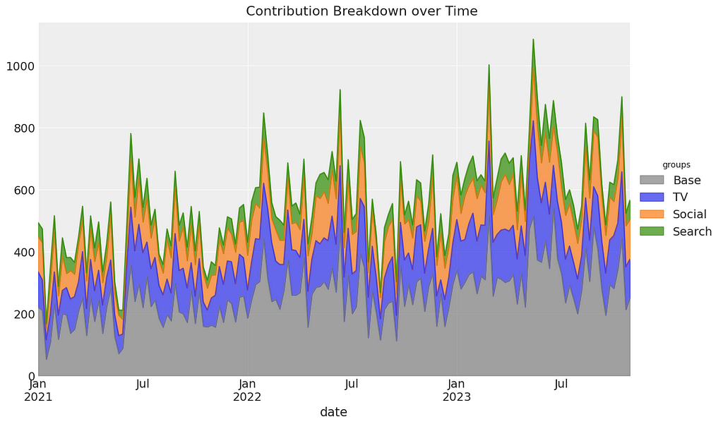
Welcome to part 1 of my series on marketing mix modeling (MMM), a hands-on guide to help you master MMM. Throughout this series, we’ll cover key topics such as model training, validation, calibration and budget optimisation, all using the powerful pymc-marketing python package. Whether you’re new to MMM or looking to sharpen your skills, this series will equip you with practical tools and insights to improve your marketing strategies.

Introduction

In this article, we’ll start by providing some background on Bayesian MMM, including the following topics:

• What open source packages can we use?
• What is Bayesian MMM?
• What are Bayesian priors?
• Are the default priors in pymc-marketing sensible?

We will then move on to a walkthrough in Python using the pymc-marketing package, diving deep into the following areas:

• Simulating data
• Training the model
• Validating the model
• Parameter recovery

The full notebook can be found here:

pymc_marketing/notebooks/1. training marketing mix models (MMM) in python.ipynb at main · raz1470/pymc_marketing

1.0 MMM Background

Let’s begin with a brief overview of Marketing Mix Modeling (MMM). We’ll explore various open-source packages available for implementation and delve into the principles of Bayesian MMM, including the concept of priors. Finally, we’ll evaluate the default priors used in pymc-marketing to gauge their suitability and effectiveness..

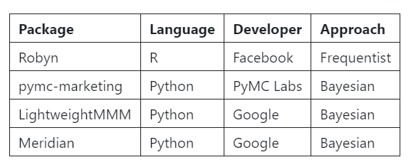
1.1 What open source packages can we use?

When it comes to MMM, there are several open-source packages we can use:

There are several compelling reasons to focus on pymc-marketing in this series:

1. Python Compatibility: Unlike Robyn, which is available only in R, pymc-marketing caters to a broader audience who prefer working in Python.
2. Current Availability: Meridian has not yet been released (as of September 23, 2024), making pymc-marketing a more accessible option right now.
3. Future Considerations: LightweightMMM is set to be decommissioned once Meridian is launched, further solidifying the need for a reliable alternative.
4. Active Development: pymc-marketing is continuously enhanced by its extensive community of contributors, ensuring it remains up-to-date with new features and improvements.

You can check out the pymc-marketing package here, they offer some great notebook to illustrate some of the packages functionality:

How-to – pymc-marketing 0.9.0 documentation

1.2 What is Bayesian MMM?

You’ll notice that 3 out of 4 of the packages highlighted above take a Bayesian approach. So let’s take a bit of time to understand what Bayesian MMM looks like! For beginners, Bayesian analysis is a bit of a rabbit hole but we can break it down into 5 key points:

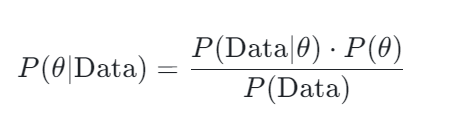
1. Bayes’ Theorem — In Bayesian MMM, Bayes’ theorem is used to update our beliefs about how marketing channels impact sales as we gather new data. For example, if we have some initial belief about how much TV advertising affects sales, Bayes’ theorem allows us to refine that belief after seeing actual data on sales and TV ad spend.
2. P(θ) — Priors represent our initial beliefs about the parameters in the model, such as the effect of TV spend on sales. For example, if we ran a geo-lift test which estimated that TV ads increase sales by 5%, we might set a prior based on that estimate.
3. P(Data | θ) — The likelihood function, which captures the probability of observing the sales data given specific levels of marketing inputs. For example, if you spent £100,000 on social media and saw a corresponding sales increase, the likelihood tells us how probable that sales jump is based on the assumed effect of social media.
4. P(θ | Data) — The posterior is what we ultimately care about in Bayesian MMM — it’s our updated belief about how different marketing channels impact sales after combining the data and our prior assumptions. For instance, after observing new sales data, our initial belief that TV ads drive a 5% increase in sales might be adjusted to a more refined estimate, like 4.7%.
5. Sampling — Since Bayesian MMM involves complex models with multiple parameters (e.g. adstock, saturation, marketing channel effects, control effects etc.) computing the posterior directly can be difficult. MCMC (Markov Chain Monte Carlo) allows us to approximate the posterior by generating samples from the distribution of each parameter. This approach is particularly helpful when dealing with models that would be hard to solve analytically.

1.3 What are Bayesian priors?

Bayesian priors are supplied as probability distributions. Instead of assigning a fixed value to a parameter, we provide a range of potential values, along with the likelihood of each value being the true one. Common distributions used for priors include:

• Normal: For parameters where we expect values to cluster around a mean.
• Half-Normal: For parameters where we want to enforce positivity.
• Beta: For parameters which are constrained between 0 and 1.
• Gamma: For parameters that are positive and skewed.

You may hear the term informative priors. Ideally, we supply these based on expert knowledge or randomized experiments. Informative priors reflect strong beliefs about the parameter values. However, when this is not feasible, we can use non-informative priors, which spread probability across a wide range of values. Non-informative priors allow the data to dominate the posterior, preventing prior assumptions from overly influencing the outcome.

1.4 Are the default priors in pymc-marketing sensible?

When using the pymc-marketing package, the default priors are designed to be weakly informative, meaning they provide broad guidance without being overly specific. Instead of being overly specific, they guide the model without restricting it too much. This balance ensures the priors guide the model without overshadowing the data..

To build reliable models, it’s crucial to understand the default priors rather than use them blindly. In the following sections, we will examine the various priors used in pymc-marketing and explain why the default choices are sensible for marketing mix models.

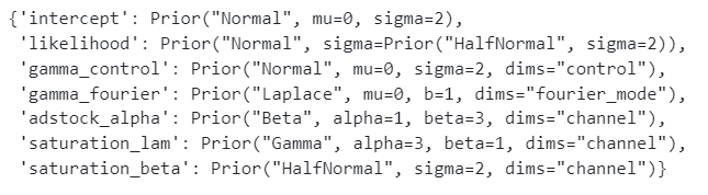
We can start by using the code below to inspect the default priors:

dummy_model = MMM(
    date_column="",
    channel_columns=[""],
    adstock=GeometricAdstock(l_max=4),
    saturation=LogisticSaturation(),
)
dummy_model.default_model_config

Above I have printed out a dictionary containing the 7 default priors — Let’s start by briefly understanding what each one is:

• intercept — The baseline level of sales or target variable in the absence of any marketing spend or other variables. It sets the starting point for the model.
• likelihood — When you increase the focus on the likelihood, the model relies more heavily on the observed data and less on the priors. This means the model will be more data-driven, allowing the observed outcomes to have a stronger influence on the parameter estimates
• gamma_control — Control variables that account for external factors, such as macroeconomic conditions, holidays, or other non-marketing variables that might influence sales.
• gamma_fourier — Fourier terms used to model seasonality in the data, capturing recurring patterns or cycles in sales.
• adstock_alpha — Controls the adstock effect, determining how much the impact of marketing spend decays over time.
• saturation_lamda — Defines the steepness of the saturation curve, determining how quickly diminishing returns set in as marketing spend increases.
• saturation_beta — The marketing spend coefficient, which measures the direct effect of marketing spend on the target variable (e.g. sales).

Next we are going to focus on gaining a more in depth understanding of parameters for marketing and control variables.

1.4.1 Adstock alpha

Adstock reflects the idea that the influence of a marketing activity is delayed and builds up over time. The adstock alpha (the decay rate) controls how quickly the effect diminishes over time, determining how long the impact of the marketing activity continues to influence sales.

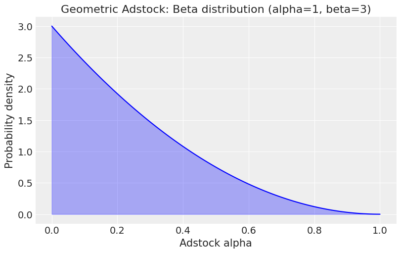
A beta distribution is used as a prior for adstock alpha. Let’s first visualise the beta distribution:

alpha = 1
beta_param = 3

x1 = np.linspace(0, 1, 100)
y1 = beta.pdf(x1, alpha, beta_param)

plt.figure(figsize=(8, 5))
plt.plot(x1, y1, color='blue')
plt.fill_between(x1, y1, color='blue', alpha=0.3)
plt.title('Geometric Adstock: Beta distribution (alpha=1, beta=3)')
plt.xlabel('Adstock alpha')
plt.ylabel('Probability density')
plt.grid(True)
plt.show()

We typically constrain adstock alpha values between 0 and 1, making the beta distribution a sensible choice. Specifically, using a beta(1, 3) prior for adstock alpha reflects the belief that, in most cases, the decay rate should be relatively high, meaning the effect of marketing activities wears off quickly.

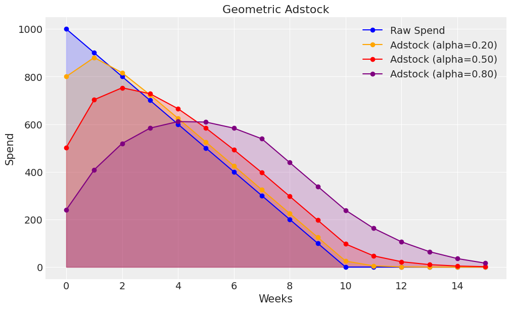
To build further intuition, we can visualise the effect of different adstock alpha values:

raw_spend = np.array([1000, 900, 800, 700, 600, 500, 400, 300, 200, 100, 0, 0, 0, 0, 0, 0])

adstock_spend_1 = geometric_adstock(x=raw_spend, alpha=0.20, l_max=8, normalize=True).eval().flatten()
adstock_spend_2 = geometric_adstock(x=raw_spend, alpha=0.50, l_max=8, normalize=True).eval().flatten()
adstock_spend_3 = geometric_adstock(x=raw_spend, alpha=0.80, l_max=8, normalize=True).eval().flatten()

plt.figure(figsize=(10, 6))

plt.plot(raw_spend, marker='o', label='Raw Spend', color='blue')
plt.fill_between(range(len(raw_spend)), 0, raw_spend, color='blue', alpha=0.2)

plt.plot(adstock_spend_1, marker='o', label='Adstock (alpha=0.20)', color='orange')
plt.fill_between(range(len(adstock_spend_1)), 0, adstock_spend_1, color='orange', alpha=0.2)

plt.plot(adstock_spend_2, marker='o', label='Adstock (alpha=0.50)', color='red')
plt.fill_between(range(len(adstock_spend_2)), 0, adstock_spend_2, color='red', alpha=0.2)

plt.plot(adstock_spend_3, marker='o', label='Adstock (alpha=0.80)', color='purple')
plt.fill_between(range(len(adstock_spend_3)), 0, adstock_spend_3, color='purple', alpha=0.2)

plt.xlabel('Weeks')
plt.ylabel('Spend')
plt.title('Geometric Adstock')
plt.legend()
plt.grid(True)
plt.show()

• Low values of alpha have little impact and are suitable for channels which have a direct response e.g. paid social performance ads with a direct call to action aimed at prospects who have already visited your website.
• Higher values of alpha have a stronger impact and are suitable for channels which have a longer term effect e.g. brand building videos with no direct call to action aimed at a broad range of prospects.

1.4.2 Saturation lamda

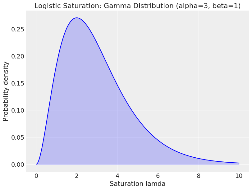
As we increase marketing spend, it’s incremental impact of sales slowly starts to reduce — This is known as saturation. Saturation lamda controls the steepness of the saturation curve, determining how quickly diminishing returns set in.

A gamma distribution is used as a prior for saturation lambda. Let’s start by understanding what a gamma distribution looks like:

alpha = 3
beta = 1

x2 = np.linspace(0, 10, 1000)
y2 = gamma.pdf(x2, alpha, scale=1/beta)

plt.figure(figsize=(8, 6))
plt.plot(x2, y2, 'b-')
plt.fill_between(x2, y2, alpha=0.2, color='blue')
plt.title('Logistic Saturation: Gamma Distribution (alpha=3, beta=1)')
plt.xlabel('Saturation lamda')
plt.ylabel('Probability density')
plt.grid(True)
plt.show()

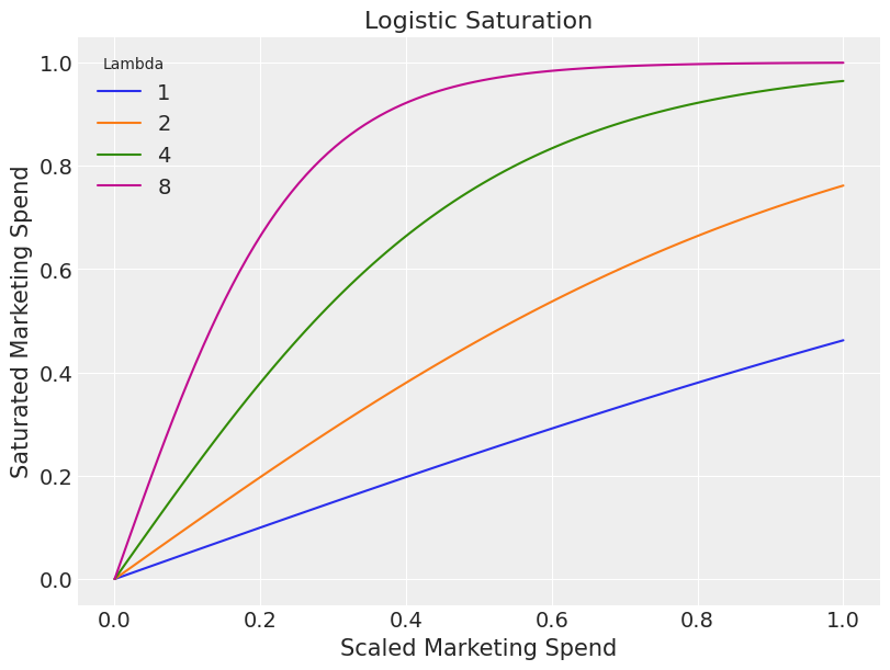
At first glance it can be difficult to understand why the gamma distribution is a sensible choice of prior but plotting the impact of different lamda values helps clarify its appropriateness::

scaled_spend = np.linspace(start=0.0, stop=1.0, num=100)

saturated_spend_1 = logistic_saturation(x=scaled_spend, lam=1).eval()
saturated_spend_2 = logistic_saturation(x=scaled_spend, lam=2).eval()
saturated_spend_4 = logistic_saturation(x=scaled_spend, lam=4).eval()
saturated_spend_8 = logistic_saturation(x=scaled_spend, lam=8).eval()

plt.figure(figsize=(8, 6))
sns.lineplot(x=scaled_spend, y=saturated_spend_1, label="1")
sns.lineplot(x=scaled_spend, y=saturated_spend_2, label="2")
sns.lineplot(x=scaled_spend, y=saturated_spend_4, label="4")
sns.lineplot(x=scaled_spend, y=saturated_spend_8, label="8")

plt.title('Logistic Saturation')
plt.xlabel('Scaled Marketing Spend')
plt.ylabel('Saturated Marketing Spend')
plt.legend(title='Lambda')
plt.grid(True)
plt.show()

• A lamda value of 1 keeps the relationship linear.
• As we increase lamda, the steepness of the saturation curve increases.
• From the chart we hopefully agree that it seems unlikely to have a saturation much steeper than what we see when the lamda value is 8.

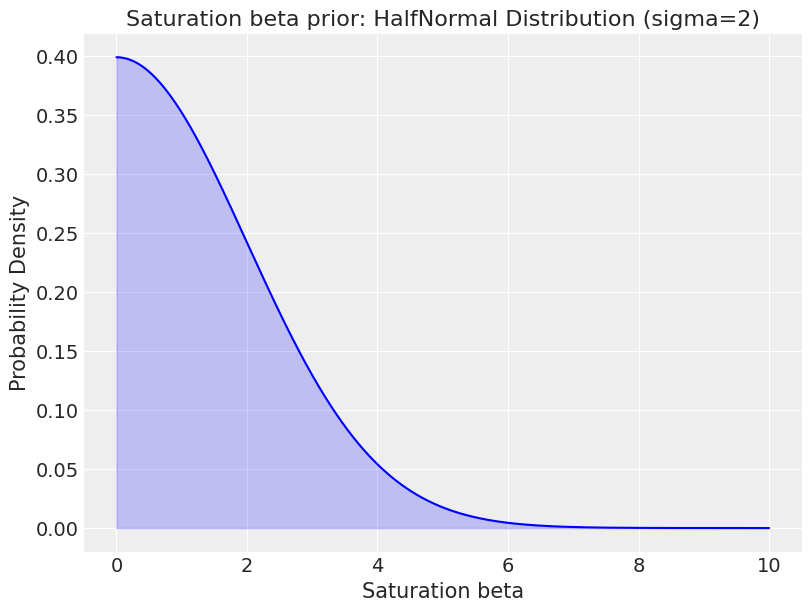
1.4.3 Saturation beta

Saturation beta corresponds to the marketing channel coefficient, measuring the impact of marketing spend.

The half-normal prior is used as it enforces positivity which is a very reasonable assumption e.g. marketing shouldn’t have a negative effect. When sigma is set as 2, it tends towards low values. This helps regularize the coefficients, pulling them towards lower values unless there is strong evidence in the data that a particular channel has a significant impact.

sigma = 2

x3 = np.linspace(0, 10, 1000)
y3 = halfnorm.pdf(x3, scale=sigma)

plt.figure(figsize=(8, 6))
plt.plot(x3, y3, 'b-')
plt.fill_between(x3, y3, alpha=0.2, color='blue')
plt.title('Saturation beta prior: HalfNormal Distribution (sigma=2)')
plt.xlabel('Saturation beta')
plt.ylabel('Probability Density')
plt.grid(True)
plt.show()

Remember that both the marketing and target variables are scaled (ranging from 0 to 1), so the beta prior must be in this scaled space.

1.4.4 Gamma control

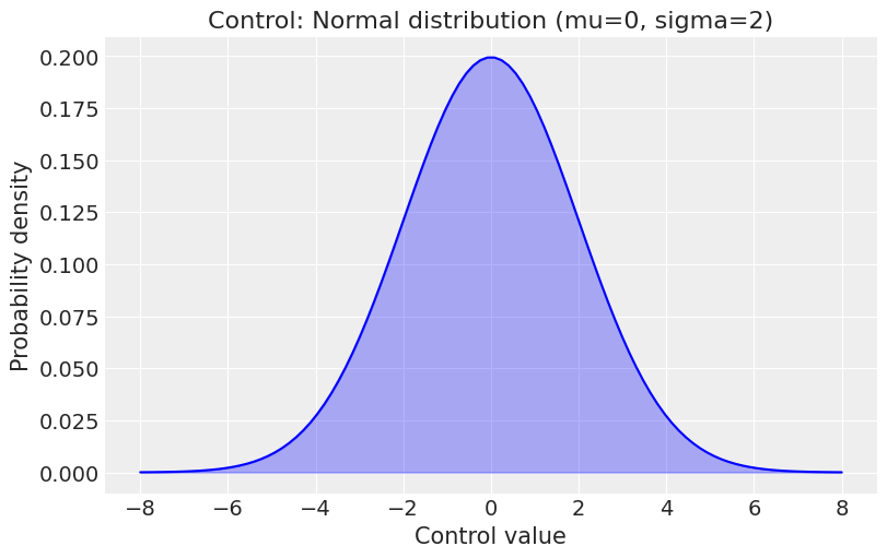
The gamma control parameter is the coefficient for the control variables that account for external factors, such as macroeconomic conditions, holidays, or other non-marketing variables.

A normal distribution is used which allows for both positive and negative effects:

mu = 0
sigma = 2

x = np.linspace(mu - 4*sigma, mu + 4*sigma, 100)
y = norm.pdf(x, mu, sigma)

plt.figure(figsize=(8, 5))
plt.plot(x, y, color='blue')
plt.fill_between(x, y, color='blue', alpha=0.3)
plt.title('Control: Normal distribution (mu=0, sigma=2)')
plt.xlabel('Control value')
plt.ylabel('Probability density')
plt.grid(True)
plt.show()

Control variables are standardized, with values ranging from -1 to 1, so the gamma control prior must be in this scaled space.

2.0 Python Walkthrough

Now we have covered some of the theory, let’s but some of it into practice! In this walkthrough we will cover:

• Simulating data
• Training the model
• Validating the model
• Parameter recovery

The aim is to create some realistic training data where we set the parameters ourselves (adstock, saturation, beta etc.), train and validate a model utilising the pymc-marketing package, and then assess how well our model did at recovering the parameters.

When it comes to real world MMM data, you won’t know the parameters, but this exercise of parameter recovery is a great way to learn and get confident in MMM.

2.1 Simulating data

Let’s start by simulating some data to train a model. The benefit of this approach is that we can set the parameters ourselves, which allows us to conduct a parameter recovery exercise to test how well our model performs!

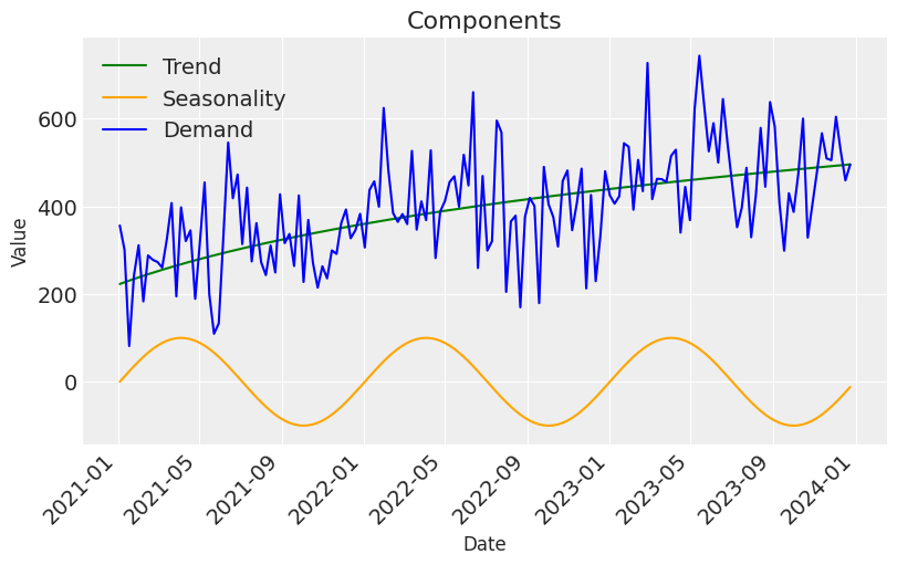
The function below can be used to simulate some data with the following characteristics:

1. A trend component with some growth.
2. A seasonal component with oscillation around 0.
3. The trend and seasonal component are used to create demand.
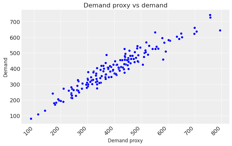
4. A proxy for demand is created which will be available for the model (demand will be an unobserved confounder).
5. Demand is a key driver of sales.
6. Each marketing channel also contributes to sales, the marketing spend is correlated with demand and the appropriate transformation are applied (scaling, adstock, saturation).

import pandas as pd
import numpy as np
from pymc_marketing.mmm.transformers import geometric_adstock, logistic_saturation
from sklearn.preprocessing import MaxAbsScaler

def data_generator(start_date, periods, channels, spend_scalar, adstock_alphas, saturation_lamdas, betas, freq="W"):
    '''
    Generates a synthetic dataset for a MMM with trend, seasonality, and channel-specific contributions.

    Args:
        start_date (str or pd.Timestamp): The start date for the generated time series data.
        periods (int): The number of time periods (e.g., days, weeks) to generate data for.
        channels (list of str): A list of channel names for which the model will generate spend and sales data.
        spend_scalar (list of float): Scalars that adjust the raw spend for each channel to a desired scale.
        adstock_alphas (list of float): The adstock decay factors for each channel, determining how much past spend influences the current period.
        saturation_lamdas (list of float): Lambda values for the logistic saturation function, controlling the saturation effect on each channel.
        betas (list of float): The coefficients for each channel, representing the contribution of each channel's impact on sales.

    Returns:
        pd.DataFrame: A DataFrame containing the generated time series data, including demand, sales, and channel-specific metrics.
    '''
    
    # 0. Create time dimension
    date_range = pd.date_range(start=start_date, periods=periods, freq=freq)
    df = pd.DataFrame({'date': date_range})
    
    # 1. Add trend component with some growth
    df["trend"]= (np.linspace(start=0.0, stop=20, num=periods) + 5) ** (1 / 8) - 1
    
    # 2. Add seasonal component with oscillation around 0
    df["seasonality"] = df["seasonality"] = 0.1 * np.sin(2 * np.pi * df.index / 52)
    
    # 3. Multiply trend and seasonality to create overall demand with noise
    df["demand"] = df["trend"] * (1 + df["seasonality"]) + np.random.normal(loc=0, scale=0.10, size=periods)
    df["demand"] = df["demand"] * 1000
    
    # 4. Create proxy for demand, which is able to follow demand but has some noise added
    df["demand_proxy"] = np.abs(df["demand"]* np.random.normal(loc=1, scale=0.10, size=periods))
    
    # 5. Initialize sales based on demand
    df["sales"] = df["demand"]
    
    # 6. Loop through each channel and add channel-specific contribution
    for i, channel in enumerate(channels):
        
        # Create raw channel spend, following demand with some random noise added
        df[f"{channel}_spend_raw"] = df["demand"] * spend_scalar[i]
        df[f"{channel}_spend_raw"] = np.abs(df[f"{channel}_spend_raw"] * np.random.normal(loc=1, scale=0.30, size=periods))
               
        # Scale channel spend
        channel_transformer = MaxAbsScaler().fit(df[f"{channel}_spend_raw"].values.reshape(-1, 1))
        df[f"{channel}_spend"] = channel_transformer .transform(df[f"{channel}_spend_raw"].values.reshape(-1, 1))
        
        # Apply adstock transformation
        df[f"{channel}_adstock"] = geometric_adstock(
            x=df[f"{channel}_spend"].to_numpy(),
            alpha=adstock_alphas[i],
            l_max=8, normalize=True
        ).eval().flatten()
        
        # Apply saturation transformation
        df[f"{channel}_saturated"] = logistic_saturation(
            x=df[f"{channel}_adstock"].to_numpy(),
            lam=saturation_lamdas[i]
        ).eval()
        
        # Calculate contribution to sales
        df[f"{channel}_sales"] = df[f"{channel}_saturated"] * betas[i]
        
        # Add the channel-specific contribution to sales
        df["sales"] += df[f"{channel}_sales"]
    
    return df

We can now call the data generator function with some parameters which are realistic:

• 3 years of weekly data.
• 3 channels from different parts of the marketing funnel.
• Each channel has a different adstock, saturation and beta parameter.

np.random.seed(10)

# Set parameters for data generator
start_date = "2021-01-01"
periods = 52 * 3
channels = ["tv", "social", "search"]
adstock_alphas = [0.50, 0.25, 0.05]
saturation_lamdas = [1.5, 2.5, 3.5]
betas = [350, 150, 50]
spend_scalars = [10, 15, 20]

df = dg.data_generator(start_date, periods, channels, spend_scalars, adstock_alphas, saturation_lamdas, betas)

# Scale betas using maximum sales value - this is so it is comparable to the fitted beta from pymc (pymc does feature and target scaling using MaxAbsScaler from sklearn)
betas_scaled = [
    ((df["tv_sales"] / df["sales"].max()) / df["tv_saturated"]).mean(),
    ((df["social_sales"] / df["sales"].max()) / df["social_saturated"]).mean(),
    ((df["search_sales"] / df["sales"].max()) / df["search_saturated"]).mean()
]

# Calculate contributions - these will be used later on to see how accurate the contributions from our model are
contributions = np.asarray([
    round((df["tv_sales"].sum() / df["sales"].sum()), 2),
    round((df["social_sales"].sum() / df["sales"].sum()), 2),
    round((df["search_sales"].sum() / df["sales"].sum()), 2),
    round((df["demand"].sum() / df["sales"].sum()), 2)
])

df[["date", "demand", "demand_proxy", "tv_spend_raw", "social_spend_raw", "search_spend_raw", "sales"]]

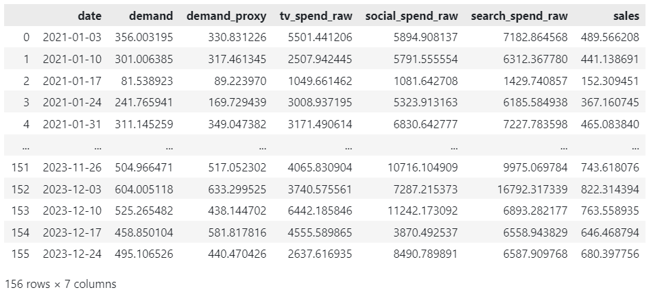
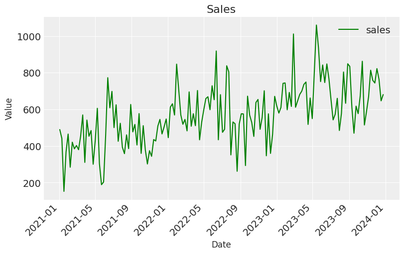
Before we move onto training a model, let’s spend some time understanding the data we have generated.

• The intuition behind how we have derived demand is that there has been an increasing trend for organic growth, with the addition of a high and low demand period each year.

plt.figure(figsize=(8, 5))

sns.lineplot(x=df['date'], y=df['trend']*1000, label="Trend", color="green")
sns.lineplot(x=df['date'], y=df['seasonality']*1000, label="Seasonality", color="orange")
sns.lineplot(x=df['date'], y=df['demand'], label="Demand", color="blue")

plt.title('Components', fontsize=16)
plt.xlabel('Date', fontsize=12)
plt.ylabel('Value', fontsize=12)
plt.xticks(rotation=45, ha='right')
plt.legend()
plt.show()

• We created a proxy for demand to be used as a control variable in the model. The idea here is that, in reality demand is an unobserved confounder, but we can sometimes find proxies for demand. One example of this is google search trends data for the product you are selling.

plt.figure(figsize=(8, 5))

sns.scatterplot(x=df['demand_proxy'], y=df['demand'], color="blue")

plt.title('Demand proxy vs demand', fontsize=16)
plt.xlabel('Demand proxy', fontsize=12)
plt.ylabel('Demand', fontsize=12)
plt.xticks(rotation=45, ha='right')
plt.show()

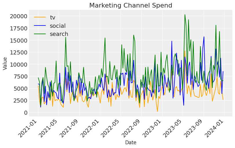
• Spend follows the same trend for each marketing channel but the random noise we added should allow the model to unpick how each one is contributing to sales.

plt.figure(figsize=(8, 5))

sns.lineplot(x=df['date'], y=df['tv_spend_raw'], label=channels[0], color="orange")
sns.lineplot(x=df['date'], y=df['social_spend_raw'], label=channels[1], color="blue")
sns.lineplot(x=df['date'], y=df['search_spend_raw'], label=channels[2], color="green")
plt.title('Marketing Channel Spend', fontsize=16)
plt.xlabel('Date', fontsize=12)
plt.ylabel('Value', fontsize=12)
plt.xticks(rotation=45, ha='right')
plt.legend()
plt.show()

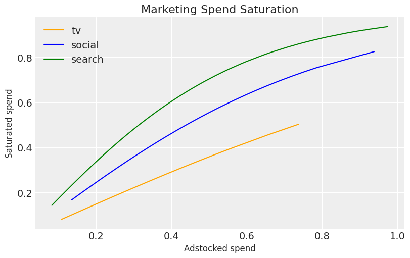
• We applied two transformation to our marketing data, adstock and saturation. Below we can look at the effect of the different parameters we used for each channels saturation, with search having the steepest saturation and TV almost being linear.

plt.figure(figsize=(8, 5))

sns.lineplot(x=df['tv_adstock'], y=df['tv_saturated'], label=channels[0], color="orange")
sns.lineplot(x=df['social_adstock'], y=df['social_saturated'], label=channels[1], color="blue")
sns.lineplot(x=df['search_adstock'], y=df['search_saturated'], label=channels[2], color="green")

plt.title('Marketing Spend Saturation', fontsize=16)
plt.xlabel('Adstocked spend', fontsize=12)
plt.ylabel('Saturated spend', fontsize=12)
plt.legend()
plt.show()

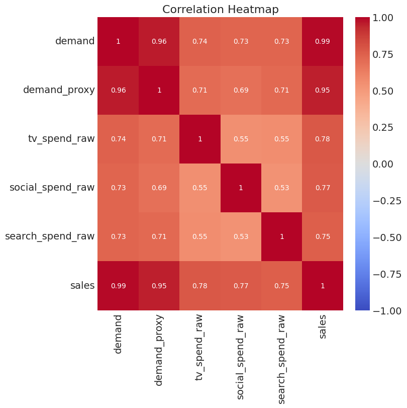
• Below we can see that our variables are highly correlated, something that is very common in MMM data due to marketing teams spending more in peak periods.

plt.figure(figsize=(8, 8))
sns.heatmap(df[["demand", "demand_proxy", "tv_spend_raw", "social_spend_raw", "search_spend_raw", "sales"]].corr(), annot=True, cmap='coolwarm', vmin=-1, vmax=1)
plt.title('Correlation Heatmap')
plt.show()

• And finally let’s take a look at sales — Remember our aim is to understand how marketing has contributed to sales.

plt.figure(figsize=(8, 5))

sns.lineplot(x=df['date'], y=df['sales'], label="sales", color="green")

plt.title('Sales', fontsize=16)
plt.xlabel('Date', fontsize=12)
plt.ylabel('Value', fontsize=12)
plt.xticks(rotation=45, ha='right')
plt.legend()
plt.show()

Now that we have a good understanding of the data generating process, let’s dive into training the model!

2.2 Training the model

It’s now time to move on to training the model. To begin with we need to prepare the training data by:

• Splitting data into features and target.
• Creating indices for train and out-of-time slices — The out-of-time slice will help us validate our model.

# set date column
date_col = "date"

# set outcome column
y_col = "sales"

# set marketing variables
channel_cols = ["tv_spend_raw",
                "social_spend_raw",
                "search_spend_raw"]

# set control variables
control_cols = ["demand_proxy"]

# split data into features and target
X = df[[date_col] + channel_cols + control_cols]
y = df[y_col]

# set test (out-of-sample) length
test_len = 8

# create train and test indices
train_idx = slice(0, len(df) - test_len)
out_of_time_idx = slice(len(df) - test_len, len(df))

Next we initiate the MMM class. A major challenge in MMM is the fact that the ratio of parameters to training observations is high. One way we can mitigate this is by being pragmatic about the choice of transformations:

• We select geometric adstock which has 1 parameter (per channel) vs 2 compared to using weibull adstock.
• We select logistic saturation which has 1 parameter (per channel) vs 2 compared to using hill saturation.
• We use a proxy for demand and decide not to include a seasonal component or time varying trend which further reduces our parameters.
• We decide not to include time varying media parameters on the basis that, although it is true that performance varies over time, we ultimately want a response curve to help us optimise budgets and taking the average performance over the training dataset is a good way to do this.

To summarise my view here, the more complexity we add to the model, the more we manipulate our marketing spend variables to fit the data which in turn gives us a “better model” (e.g. high R-squared and low mean squared error). But this is at the risk of moving away from the true data generating process which in-turn will give us biased causal effect estimates.

mmm_default = MMM(
    adstock=GeometricAdstock(l_max=8),
    saturation=LogisticSaturation(),
    date_column=date_col,
    channel_columns=channel_cols,
    control_columns=control_cols,
)

mmm_default.default_model_config

Now let’s fit the model using the train indices. I’ve passed some optional key-word-arguments, let’s spend a bit of time understanding what they do:

• Tune — This sets the number of tuning steps for the sampler. During tuning, the sampler adjusts its parameters to efficiently explore the posterior distribution. These initial 1,000 samples are discarded and not used for inference.
• Chains — This specifies the number of independent Markov chains to run. Running multiple chains helps assess convergence and provides a more robust sampling of the posterior.
• Draws — This sets the number of samples to draw from the posterior distribution per chain, after tuning.
• Target accept — This is the target acceptance rate for the sampler. It helps balance exploration of the parameter space with efficiency.

fit_kwargs = {
    "tune": 1_000,
    "chains": 4,
    "draws": 1_000,
    "target_accept": 0.9,
}

mmm_default.fit(X[train_idx], y[train_idx], **fit_kwargs)

I’d advise sticking with the defaults here, and only changing them if you get some issues in the next steps in terms of divergences.

2.3 Validating the model

After fitting the model, the first step is to check for divergences. Divergences indicate potential problems with either the model or the sampling process. Although delving deeply into divergences is beyond the scope of this article due to its complexity, it’s essential to note their importance in model validation.

Below, we check the number of divergences in our model. A result of 0 divergences indicates a good start.

mmm_default.idata["sample_stats"]["diverging"].sum().item()

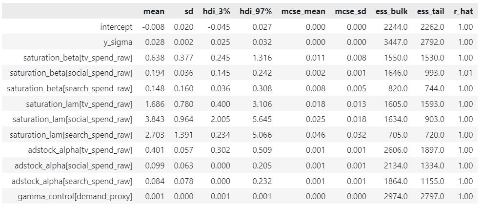
Next we can get a comprehensive summary of the MCMC sampling results. Let’s focus on the key ones:

• mean — The average value of the parameter across all samples.
• hdi_3% and hdi_97% — The lower and upper bounds of the 94% Highest Density Interval (HDI). A 94% HDI means that there’s a 94% probability that the true value of the parameter lies within this interval, based on the observed data and prior information.
• rhat — Gelman-Rubin statistic, measuring convergence across chains. Values close to 1 (typically < 1.05) indicate good convergence.

Our R-hats are all very close to 1, which is expected given the absence of divergences. We will revisit the mean parameter values in the next section when we conduct a parameter recovery exercise.

az.summary(
    data=mmm_default.fit_result,
    var_names=[
        "intercept",
        "y_sigma",
        "saturation_beta",
        "saturation_lam",
        "adstock_alpha",
        "gamma_control",
    ],
)

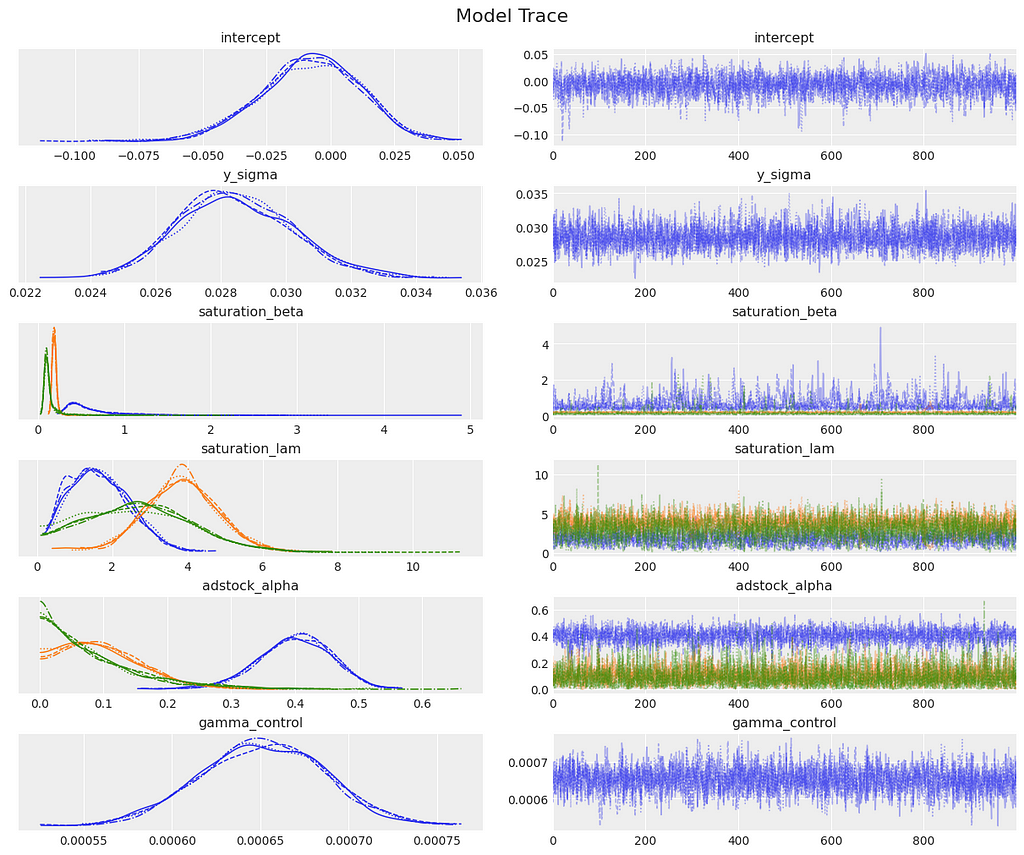
Next, we generate diagnostic plots that are crucial for assessing the quality of our MCMC sampling:

• Posterior Distribution (left): Displays the value of each parameter throughout the MCMC sampling. Ideally, these should be smooth and unimodal, with all chains showing similar distributions.
• Trace Plots (right): Illustrate the value of each parameter over the MCMC sampling process. Any trends or slow drifts may indicate poor mixing or non-convergence, while chains that don’t overlap could suggest they are stuck in different modes of the posterior.

Looking at our diagnostic plots there are no red flags.

_ = az.plot_trace(
    data=mmm_default.fit_result,
    var_names=[
        "intercept",
        "y_sigma",
        "saturation_beta",
        "saturation_lam",
        "adstock_alpha",
        "gamma_control",
    ],
    compact=True,
    backend_kwargs={"figsize": (12, 10), "layout": "constrained"},
)
plt.gcf().suptitle("Model Trace", fontsize=16);

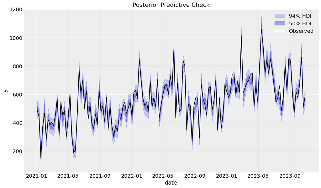
For each parameter we have a distribution of possible values which reflects the uncertainty in the parameter estimates. For the next set of diagnostics, we first need to sample from the posterior. This allows us to make predictions, which we will do for the training data.

mmm_default.sample_posterior_predictive(X[train_idx], extend_idata=True, combined=True)

We can begin the posterior predictive checking diagnostics by visually assessing whether the observed data falls within the predicted ranges. It appears that our model has performed well.

mmm_default.plot_posterior_predictive(original_scale=True);

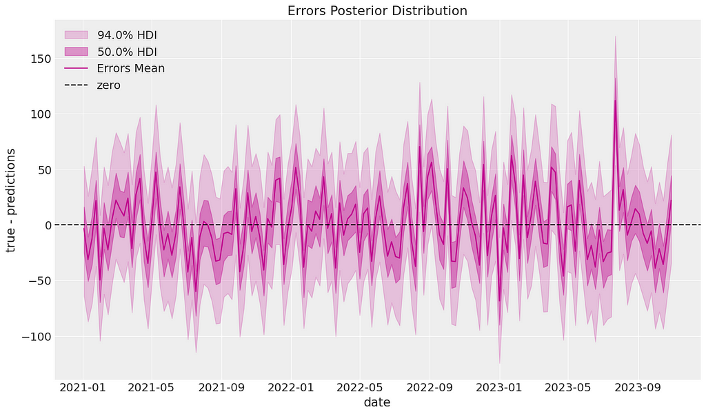
Next we can calculate residuals between the posterior predictive mean and the actual data. We can plot these residuals over time to check for patterns or autocorrelation. It looks like the residuals oscillate around 0 as expected.

mmm_default.plot_errors(original_scale=True);

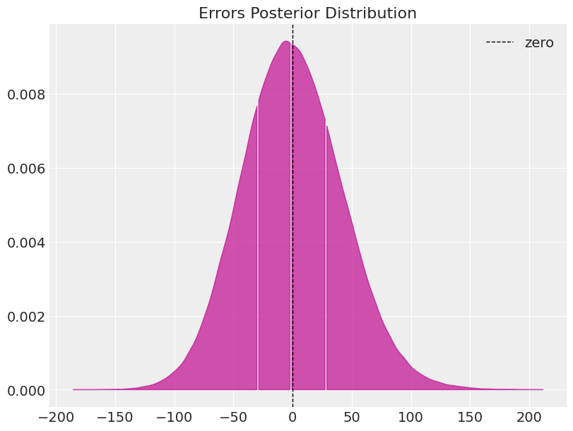
We can also check whether the residuals are normally distributed around 0. Again, we pass this diagnostic test.

errors = mmm_default.get_errors(original_scale=True)

fig, ax = plt.subplots(figsize=(8, 6))
az.plot_dist(
    errors, quantiles=[0.25, 0.5, 0.75], color="C3", fill_kwargs={"alpha": 0.7}, ax=ax
)
ax.axvline(x=0, color="black", linestyle="--", linewidth=1, label="zero")
ax.legend()
ax.set(title="Errors Posterior Distribution");

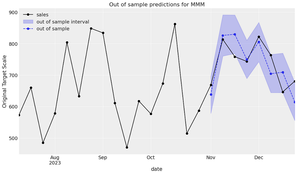
Finally it is good practice to assess how good our model is at predicting outside of the training sample. First of all we need to sample from the posterior again but this time using the out-of-time data. We can then plot the observed sales against the predicted.

Below we can see that the observed sales generally lie within the intervals and the model seems to do a good job.

y_out_of_sample = mmm_default.sample_posterior_predictive(
    X_pred=X[out_of_time_idx], extend_idata=False, include_last_observations=True
)

def plot_in_sample(X, y, ax, n_points: int = 15):
    (
        y.to_frame()
        .set_index(X[date_col])
        .iloc[-n_points:]
        .plot(ax=ax, marker="o", color="black", label="actuals")
    )
    return ax


def plot_out_of_sample(X_out_of_sample, y_out_of_sample, ax, color, label):
    y_out_of_sample_groupby = y_out_of_sample["y"].to_series().groupby("date")

    lower, upper = quantiles = [0.025, 0.975]
    conf = y_out_of_sample_groupby.quantile(quantiles).unstack()
    ax.fill_between(
        X_out_of_sample[date_col].dt.to_pydatetime(),
        conf[lower],
        conf[upper],
        alpha=0.25,
        color=color,
        label=f"{label} interval",
    )

    mean = y_out_of_sample_groupby.mean()
    mean.plot(ax=ax, marker="o", label=label, color=color, linestyle="--")
    ax.set(ylabel="Original Target Scale", title="Out of sample predictions for MMM")
    return ax


_, ax = plt.subplots()
plot_in_sample(X, y, ax=ax, n_points=len(X[out_of_time_idx])*3)
plot_out_of_sample(
    X[out_of_time_idx], y_out_of_sample, ax=ax, label="out of sample", color="C0"
)
ax.legend(loc="upper left");

Based on our findings in this section, we believe we have a robust model. In the next section let’s carry out a parameter recovery exercise to see how close to the ground truth parameters we were.

2.4 Parameter recovery

In the last section, we validated the model as we would in a real-life scenario. In this section, we will conduct a parameter recovery exercise: remember, we are only able to do this because we simulated the data ourselves and stored the true parameters.

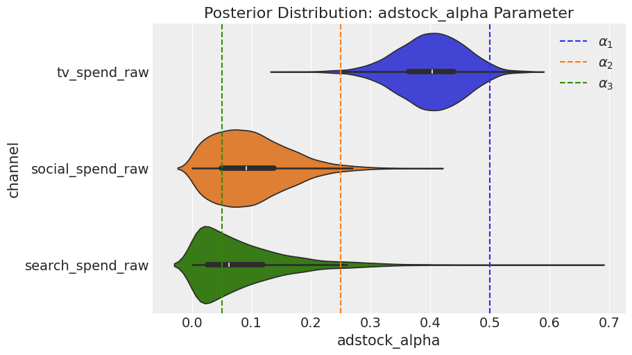
2.4.1 Parameter recovery — Adstock

Let’s begin by comparing the posterior distribution of the adstock parameters to the ground truth values that we previously stored in the adstock_alphas list. The model performed reasonably well, achieving the correct rank order, and the true values consistently lie within the posterior distribution.

fig = mmm_default.plot_channel_parameter(param_name="adstock_alpha", figsize=(9, 5))
ax = fig.axes[0]
ax.axvline(x=adstock_alphas[0], color="C0", linestyle="--", label=r"$alpha_1$")
ax.axvline(x=adstock_alphas[1], color="C1", linestyle="--", label=r"$alpha_2$")
ax.axvline(x=adstock_alphas[2], color="C2", linestyle="--", label=r"$alpha_3$")
ax.legend(loc="upper right");

2.4.2 Parameter recovery — Saturation

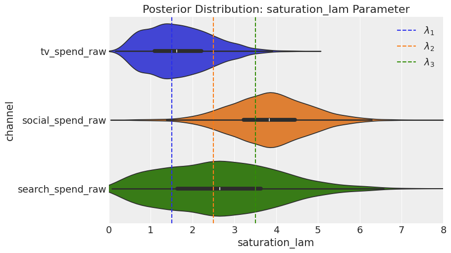
When we examine saturation, the model performs excellently in recovering lambda for TV, but it does not do as well in recovering the true values for social and search, although the results are not disastrous.

fig = mmm_default.plot_channel_parameter(param_name="saturation_lam", figsize=(9, 5))
ax = fig.axes[0]
ax.axvline(x=saturation_lamdas[0], color="C0", linestyle="--", label=r"$lambda_1$")
ax.axvline(x=saturation_lamdas[1], color="C1", linestyle="--", label=r"$lambda_2$")
ax.axvline(x=saturation_lamdas[2], color="C2", linestyle="--", label=r"$lambda_3$")
ax.legend(loc="upper right");

2.4.3 Parameter recovery — Channel betas

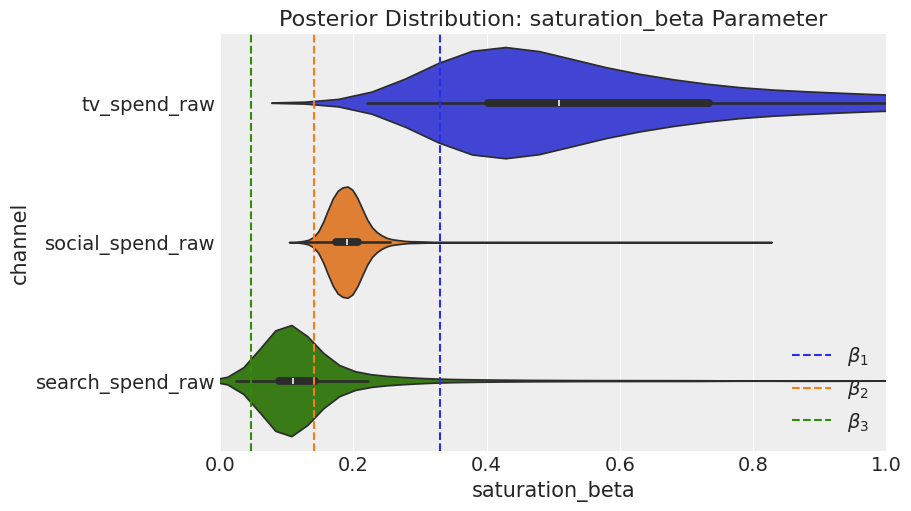
Regarding the channel beta parameters, the model achieves the correct rank ordering, but it overestimates values for all channels. In the next section, we will quantify this in terms of contribution.

fig = mmm_default.plot_channel_parameter(param_name="saturation_beta", figsize=(9, 5))
ax = fig.axes[0]
ax.axvline(x=betas_scaled[0], color="C0", linestyle="--", label=r"$beta_1$")
ax.axvline(x=betas_scaled[1], color="C1", linestyle="--", label=r"$beta_2$")
ax.axvline(x=betas_scaled[2], color="C2", linestyle="--", label=r"$beta_3$")
ax.legend(loc="upper right");

2.4.4 Parameter recovery — Channel contribution

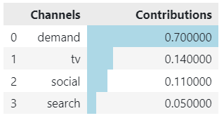
First, we calculate the ground truth contribution for each channel. We will also calculate the contribution of demand: remember we included a proxy for demand not demand itself.

channels = np.array(["tv", "social", "search", "demand"])

true_contributions = pd.DataFrame({'Channels': channels, 'Contributions': contributions})
true_contributions= true_contributions.sort_values(by='Contributions', ascending=False).reset_index(drop=True)
true_contributions = true_contributions.style.bar(subset=['Contributions'], color='lightblue')

true_contributions

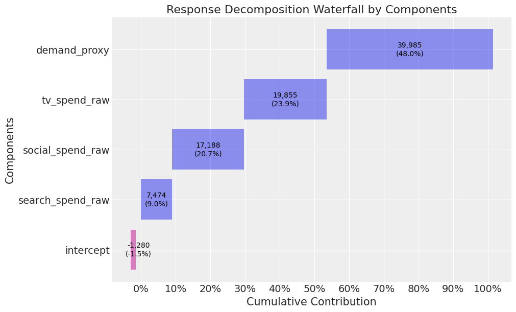
Now, let’s plot the contributions from the model. The rank ordering for demand, TV, social, and search is correct. However, TV, social, and search are all overestimated. This appears to be driven by the demand proxy not contributing as much as true demand.

mmm_default.plot_waterfall_components_decomposition(figsize=(10,6));

Closing thoughts

In section 2.3, we validated the model and concluded that it was robust. However, the parameter recovery exercise demonstrated that our model considerably overestimates the effect of marketing. This overestimation is driven by the confounding factor of demand. In a real-life scenario, it is not possible to run a parameter recovery exercise. So, how would you identify that your model’s marketing contributions are biased? And once identified, how would you address this issue? This leads us to our next article on calibrating models!

I hope you enjoyed this first instalment! Follow me if you want to continue this path towards mastering MMM — In the next article we will shift our focus to calibrating our models using informative priors from experiments.

---

Mastering Marketing Mix Modelling In Python was originally published in Towards Data Science on Medium, where people are continuing the conversation by highlighting and responding to this story.