Blog

Accelerating AI/ML Model Training with Custom Operators — Part 3.A

This is a direct sequel to a previous post on the topic of implementing custom TPU operations with Pallas. Of particular interest are custom kernels that leverage the unique properties of the TPU architecture in a manner that optimizes runtime performance. In this post, we will attempt to demonstrate this opportunity by applying the power of Pallas to the challenge of running sequential algorithms that are interspersed within a predominantly parallelizable deep learning (DL) workload.

We will focus on Non Maximum Suppression (NMS) of bounding-box proposals as a representative algorithm, and explore ways to optimize its implementation. An important component of computer vision (CV) object detection solutions (e.g., Mask RCNN), NMS is commonly used to filter out overlapping bounding boxes, keeping only the “best” ones. NMS receives a list of bounding box proposals, an associated list of scores, and an IOU threshold, and proceeds to greedily and iteratively choose the remaining box with the highest score and disqualify all other boxes with which it has an IOU that exceeds the given threshold. The fact that the box chosen at the n-th iteration depends on the preceding n-1 steps of the algorithm dictates the sequential nature of its implementation. Please see here and/or here for more on the rational behind NMS and its implementation. Although we have chosen to focus on one specific algorithm, most of our discussion should carry over to other sequential algorithms.

Offloading Sequential Algorithms to CPU

The presence of a sequential algorithm within a predominantly parallelizable ML model (e.g., Mask R-CNN) presents an interesting challenge. While GPUs, commonly used for such workloads, excel at executing parallel operations like matrix multiplication, they can significantly underperform compared to CPUs when handling sequential algorithms. This often leads to computation graphs that include crossovers between the GPU and CPU, where the GPU handles the parallel operations and the CPU handles the sequential ones. NMS is a prime example of a sequential algorithm that is commonly offloaded onto the CPU. In fact, a close analysis of torchvision’s “CUDA” implementation of NMS, reveals that even it runs a significant portion of the algorithm on CPU.

Although offloading sequential operations to the CPU may lead to improved runtime performance, there are several potential drawbacks to consider:

1. Cross-device execution between the CPU and GPU usually requires multiple points of synchronization between the devices which commonly results in idle time on the GPU while it waits for the CPU to complete its tasks. Given that the GPU is typically the most expensive component of the training platform our goal is to minimize such idle time.
2. In standard ML workflows, the CPU is responsible for preparing and feeding data to the model, which resides on the GPU. If the data input pipeline involves compute-intensive processing, this can strain the CPU, leading to “input starvation” on the GPU. In such scenarios, offloading portions of the model’s computation to the CPU could further exacerbate this issue.

To avoid these drawbacks you could consider alternative approaches, such as replacing the sequential algorithm with a comparable alternative (e.g., the one suggested here), settling for a slow/suboptimal GPU implementation of the sequential algorithm, or running the workload on CPU — each of which come with there own potential trade-offs.

Sequential Algorithms on TPU

This is where the unique architecture of the TPU could present an opportunity. Contrary to GPUs, TPUs are sequential processors. While their ability to run highly vectorized operations makes them competitive with GPUs when running parallelizable operations such as matrix multiplication, their sequential nature could make them uniquely suited for running ML workloads that include a mix of both sequential and parallel components. Armed with the Pallas extension to JAX, our newfound TPU kernel creation tool, we will evaluate this opportunity by implementing and evaluating a custom implementation of NMS for TPU.

Disclaimers

The NMS implementations we will share below are intended for demonstrative purposes only. We have not made any significant effort to optimize them or to verify their robustness, durability, or accuracy. Please keep in mind that, as of the time of this writing, Pallas is an experimental feature — still under active development. The code we share (based on JAX version 0.4.32) may become outdated by the time you read this. Be sure to refer to the most up-to-date APIs and resources available for your Pallas development. Please do not view our mention of any algorithm, library, or API as an endorsement for their use.

NMS on CPU

We begin with a simple implementation of NMS in numpy that will serve as a baseline for performance comparison:

import numpy as np

def nms_cpu(boxes, scores, max_output_size, threshold=0.1):
    epsilon = 1e-5

    # Convert bounding boxes and scores to numpy
    boxes = np.array(boxes)
    scores = np.array(scores)

    # coordinates of bounding boxes
    start_x = boxes[:, 0]
    start_y = boxes[:, 1]
    end_x = boxes[:, 2]
    end_y = boxes[:, 3]

    # Compute areas of bounding boxes
    areas = (end_x - start_x) * (end_y - start_y)

    # Sort by confidence score of bounding boxes
    order = np.argsort(scores)

    # Picked bounding boxes
    picked_boxes = []

    # Iterate over bounding boxes
    while order.size > 0 and len(picked_boxes) < max_output_size:
        
        # The index of the remaining box with the highest score
        index = order[-1]

        # Pick the bounding box with largest confidence score
        picked_boxes.append(index.item())

        # Compute coordinates of intersection
        x1 = np.maximum(start_x[index], start_x[order[:-1]])
        x2 = np.minimum(end_x[index], end_x[order[:-1]])
        y1 = np.maximum(start_y[index], start_y[order[:-1]])
        y2 = np.minimum(end_y[index], end_y[order[:-1]])

        # Compute areas of intersection and union
        w = np.maximum(x2 - x1, 0.0)
        h = np.maximum(y2 - y1, 0.0)

        intersection = w * h
        union = areas[index] + areas[order[:-1]] - intersection

        # Compute the ratio between intersection and union
        ratio = intersection / np.clip(union, min=epsilon)

        # discard boxes above overlap threshold
        keep = np.where(ratio < threshold)
        order = order[keep]

    return picked_boxes

To evaluate the performance of our NMS function, we generate a batch of random boxes and scores (as JAX tensors) and run the script on a Google Cloud TPU v5e system using the same environment and same benchmarking utility as in our previous post. For this experiment, we specify the CPU as the JAX default device:

import jax
from jax import random
import jax.numpy as jnp

def generate_random_boxes(run_on_cpu = False):
    if run_on_cpu:
        jax.config.update('jax_default_device', jax.devices('cpu')[0])
    else:
        jax.config.update('jax_default_device', jax.devices('tpu')[0])

    n_boxes = 1024
    img_size = 1024

    k1, k2, k3 = random.split(random.key(0), 3)

    # Randomly generate box sizes and positions
    box_sizes = random.randint(k1,
                               shape=(n_boxes, 2),
                               minval=1,
                               maxval=img_size)
    top_left = random.randint(k2,
                              shape=(n_boxes, 2),
                              minval=0,
                              maxval=img_size - 1)
    bottom_right = jnp.clip(top_left + box_sizes, 0, img_size - 1)

    # Concatenate top-left and bottom-right coordinates
    rand_boxes = jnp.concatenate((top_left, bottom_right),
                                 axis=1).astype(jnp.bfloat16)
    rand_scores = jax.random.uniform(k3, 
                                     shape=(n_boxes,),
                                     minval=0.0,
                                     maxval=1.0)

    return rand_boxes, rand_scores

rand_boxes, rand_scores = generate_random_boxes(run_on_cpu=True)

time = benchmark(nms_cpu)(rand_boxes, rand_scores, max_output_size=128)
print(f'nms_cpu: {time}')

The resultant average runtime is 2.99 milliseconds. Note the assumption that the input and output tensors reside on the CPU. If they are on the TPU, then the time to copy them between the devices should also be taken into consideration.

NMS on TPU

If our NMS function is a component within a larger computation graph running on the TPU, we might prefer a TPU-compatible implementation to avoid the drawbacks of cross-device execution. The code block below contains a JAX implementation of NMS specifically designed to enable acceleration via JIT compilation. Denoting the number of boxes by N, we begin by calculating the IOU between each of the N(N-1) pairs of boxes and preparing an NxN boolean tensor (mask_threshold) where the (i,j)-th entry indicates whether the IOU between boxes i and j exceed the predefined threshold.

To simplify the iterative selection of boxes, we create a copy of the mask tensor (mask_threshold2) where the diagonal elements are zeroed to prevent a box from suppressing itself. We further define two score-tracking tensors: out_scores, which retains the scores of the chosen boxes (and zeros the scores of the eliminated ones), and remaining_scores, which maintains the scores of the boxes still being considered. We then use the jax.lax.while_loop function to iteratively choose boxes while updating the out_scores and remaining_scores tensors. Note that the format of the output of this function differs from the previous function and may need to be adjusted to fit into subsequent steps of the computation graph.

import functools

# Given N boxes, calculates mask_threshold an NxN boolean mask
# where the (i,j) entry indicates whether the IOU of boxes i and j
# exceed the threshold. Returns mask_threshold, mask_threshold2
# which is equivalent to mask_threshold with zero diagonal and
# the scores modified so that all values are greater than 0
def init_tensors(boxes, scores, threshold=0.1):
    epsilon = 1e-5

    # Extract left, top, right, bottom coordinates
    left = boxes[:, 0]
    top = boxes[:, 1]
    right = boxes[:, 2]
    bottom = boxes[:, 3]

    # Compute areas of boxes
    areas = (right - left) * (bottom - top)

    # Calculate intersection points
    inter_l = jnp.maximum(left[None, :], left[:, None])
    inter_t = jnp.maximum(top[None, :], top[:, None])
    inter_r = jnp.minimum(right[None, :], right[:, None])
    inter_b = jnp.minimum(bottom[None, :], bottom[:, None])

    # Width, height, and area of the intersection
    inter_w = jnp.clip(inter_r - inter_l, 0)
    inter_h = jnp.clip(inter_b - inter_t, 0)
    inter_area = inter_w * inter_h

    # Union of the areas
    union = areas[None, :] + areas[:, None] - inter_area

    # IoU calculation
    iou = inter_area / jnp.clip(union, epsilon)

    # Shift scores to be greater than zero
    out_scores = scores - jnp.min(scores) + epsilon

    # Create mask based on IoU threshold
    mask_threshold = iou > threshold

    # Create mask excluding diagonal (i.e., self IoU is ignored)
    mask_threshold2 = mask_threshold * (1-jnp.eye(mask_threshold.shape[0],
                                                  dtype=mask_threshold.dtype))

    return mask_threshold, mask_threshold2, out_scores

@functools.partial(jax.jit, static_argnames=['max_output_size', 'threshold'])
def nms_jax(boxes, scores, max_output_size, threshold=0.1):
    # initialize mask and score tensors
    mask_threshold, mask_threshold2, out_scores = init_tensors(boxes,
                                                           scores,
                                                           threshold)

    # The out_scores tensor will retain the scores of the chosen boxes
    # and zero the scores of the eliminated ones
    # remaining_scores will maintain non-zero scores for boxes that
    # have not been chosen or eliminated
    remaining_scores = out_scores.copy()

    def choose_box(state):
        i, remaining_scores, out_scores = state
        # choose index of box with highest score from remaining scores
        index = jnp.argmax(remaining_scores)
        # check validity of chosen box
        valid = remaining_scores[index] > 0
        # If valid, zero all scores with IOU greater than threshold
        # (including the chosen index)
        remaining_scores = jnp.where(mask_threshold[index] *valid,
                                     0,
                                     remaining_scores)
        # zero the scores of the eliminated tensors (not including
        # the chosen index)
        out_scores = jnp.where(mask_threshold2[index]*valid,
                               0,
                               out_scores)

        i = i + 1
        return i, remaining_scores, out_scores

    def cond_fun(state):
        i, _, _ = state
        return (i < max_output_size)

    i = 0
    state = (i, remaining_scores, out_scores)

    _, _, out_scores = jax.lax.while_loop(cond_fun, choose_box, state)

    # Output the resultant scores. To extract the chosen boxes,
    # Take the max_output_size highest scores:
    # min = jnp.minimum(jnp.count_nonzero(scores), max_output_size)
    # indexes = jnp.argsort(out_scores, descending=True)[:min]
    return out_scores

# nms_jax can be run on either the CPU the TPU
rand_boxes, rand_scores = generate_random_boxes(run_on_cpu=True)

time = benchmark(nms_jax)(rand_boxes, rand_scores, max_output_size=128)
print(f'nms_jax on CPU: {time}')

rand_boxes, rand_scores = generate_random_boxes(run_on_cpu=False)

time = benchmark(nms_jax)(rand_boxes, rand_scores, max_output_size=128)
print(f'nms_jax on TPU: {time}')

The runtimes of this implementation of NMS are 1.231 and 0.416 milliseconds on CPU and TPU, respectively.

Custom NMS Pallas Kernel

We now present a custom implementation of NMS in which we explicitly leverage the fact that on TPUs Pallas kernels are executed in a sequential manner. Our implementation uses two boolean matrix masks and two score-keeping tensors, similar to the approach in our previous function.

We define a kernel function, choose_box, responsible for selecting the next box and updating the score-keeping tensors, which are maintained in scratch memory. We invoke the kernel across a one-dimensional grid where the number of steps (i.e., the grid-size) is determined by the max_output_size parameter.

Note that due to some limitations (as of the time of this writing) on the operations supported by Pallas, some acrobatics are required to implement both the “argmax” function and the validity check for the selected boxes. For the sake of brevity, we omit the technical details and refer the interested reader to the comments in the code below.

from jax.experimental import pallas as pl
from jax.experimental.pallas import tpu as pltpu

# argmax helper function
def pallas_argmax(scores, n_boxes):
    # we assume that the index of each box is stored in the
    # least significant bits of the score (see below)
    idx = jnp.max(scores.astype(float)).astype(int) % n_boxes
    return idx

# Pallas kernel definition
def choose_box(scores, thresh_mask1, thresh_mask2, ret_scores,
               scores_scratch, remaining_scores_scratch, *, nsteps, n_boxes):
    # initialize scratch memory on first step
    @pl.when(pl.program_id(0) == 0)
    def _():
        scores_scratch[...] = scores[...]
        remaining_scores_scratch[...] = scores[...]

    remaining_scores = remaining_scores_scratch[...]

    # choose box
    idx = pallas_argmax(remaining_scores, n_boxes)

    # we use any to verfiy validity of the chosen box due
    # to limitations on indexing in pallas
    valid = (remaining_scores>0).any()

    # updating score tensors
    remaining_scores_scratch[...] = jnp.where(thresh_mask1[idx,...]*valid,
                                              0,
                                              remaining_scores)
    scores_scratch[...] = jnp.where(thresh_mask2[idx,...]*valid,
                                    0,
                                    scores_scratch[...])

    # set return value on final step
    @pl.when(pl.program_id(0) == nsteps - 1)
    def _():
        ret_scores[...] = scores_scratch[...]

@functools.partial(jax.jit, static_argnames=['max_output_size', 'threshold'])
def nms_pallas(boxes, scores, max_output_size, threshold=0.1):
    n_boxes = scores.size
    mask_threshold, mask_threshold2, scores = init_tensors(boxes, 
                                                           scores,
                                                           threshold)

    # In order to work around the Pallas argsort limitation
    # we create a new scores tensor with the same ordering of
    # the input scores tensor in which the index of each score
    # in the ordering is encoded in the least significant bits
    sorted = jnp.argsort(scores, descending=True)

    # descending integers: n_boxes-1, ..., 2, 1, 0
    descending = jnp.flip(jnp.arange(n_boxes))

    # new scores in descending with the least significant
    # bits carrying the argsort of the input scores
    ordered_scores = n_boxes * descending + sorted

    # new scores with same ordering as input scores
    scores = jnp.empty_like(ordered_scores
                            ).at[sorted].set(ordered_scores)

    grid = (max_output_size,)
    return pl.pallas_call(
        functools.partial(choose_box, 
                          nsteps=max_output_size,
                          n_boxes=n_boxes),
        grid_spec=pltpu.PrefetchScalarGridSpec(
            num_scalar_prefetch=0,
            in_specs=[
                pl.BlockSpec(block_shape=(n_boxes,)),
                pl.BlockSpec(block_shape=(n_boxes, n_boxes)),
                pl.BlockSpec(block_shape=(n_boxes, n_boxes)),
            ],
            out_specs=pl.BlockSpec(block_shape=(n_boxes,)),
            scratch_shapes=[pltpu.VMEM((n_boxes,), scores.dtype),
                            pltpu.VMEM((n_boxes,), scores.dtype)],
            grid=grid,
        ),
        out_shape=jax.ShapeDtypeStruct((n_boxes,), scores.dtype),
        compiler_params=dict(mosaic=dict(
            dimension_semantics=("arbitrary",)))
    )(scores, mask_threshold, mask_threshold2)

rand_boxes, rand_scores = generate_random_boxes(run_on_cpu=False)

time = benchmark(nms_pallas)(rand_boxes, rand_scores, max_output_size=128)
print(f'nms_pallas: {time}')

The average runtime of our custom NMS operator is 0.139 milliseconds, making it roughly three times faster than our JAX-native implementation. This result highlights the potential of tailoring the implementation of sequential algorithms to the unique properties of the TPU architecture.

Note that in our Pallas kernel implementation, we load the full input tensors into TPU VMEM memory. Given the limited the capacity of VMEM, scaling up the input size (i.e., increase the number of bounding boxes) will likely lead to memory issues. Typically, such limitations can be addressed by chunking the inputs with BlockSpecs. Unfortunately, applying this approach would break the current NMS implementation. Implementing NMS across input chunks would require a different design, which is beyond the scope of this post.

Results

The results of our experiments are summarized in the table below:

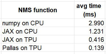
These results demonstrate the potential for running full ML computation graphs on TPU, even when they include sequential components. The performance improvement demonstrated by our Pallas NMS operator, in particular, highlights the opportunity of customizing kernels in a way that leverages the TPUs strengths.

Summary

In our previous post we learned of the opportunity for building custom TPU operators using the Pallas extension for JAX. Maximizing this opportunity requires tailoring the kernel implementations to the specific properties of the TPU architecture. In this post, we focused on the sequential nature of the TPU processor and its use in optimizing a custom NMS kernel. While scaling the solution to support an unrestricted number of bounding boxes would require further work, the core principles we have discussed remain applicable.

Still in the experimental phase of its development, there remain some limitations in Pallas that may require creative workarounds. But the strength and potential are clearly evident and we anticipate that they will only increase as the framework matures.

Implementing Sequential Algorithms on TPU was originally published in Towards Data Science on Medium, where people are continuing the conversation by highlighting and responding to this story.