Polkadot has faced strong resistance at $4.27, but the RSI shows a breakout is now possible.
The price has also touched the 50-day SMA, indicating that the short-term trend is flipping bullish.
As a machine learning engineer, I frequently see discussions on social media emphasizing the importance of deploying ML models. I completely agree — model deployment is a critical component of MLOps. As ML adoption grows, there’s a rising demand for scalable and efficient deployment methods, yet specifics often remain unclear.
So, does that mean model deployment is always the same, no matter the context? In fact, quite the opposite: I’ve been deploying ML models for about a decade now, and it can be quite different from one project to another. There are many ways to deploy a ML model, and having experience with one method doesn’t necessarily make you proficient with others.
The remaining question is: what are the methods to deploy a ML model, and how do we choose the right method?
Models can be deployed in various ways, but they typically fall into two main categories:
Cloud deployment
Edge deployment
It may sound easy, but there’s a catch. For both categories, there are actually many subcategories. Here is a non-exhaustive diagram of deployments that we will explore in this article:
Diagram of the explored subcategories of deployment in this article. Image by author.
Before talking about how to choose the right method, let’s explore each category: what it is, the pros, the cons, the typical tech stack, and I will also share some personal examples of deployments I did in that context. Let’s dig in!
Cloud Deployment
From what I can see, it seems cloud deployment is by far the most popular choice when it comes to ML deployment. This is what is usually expected to master for model deployment. But cloud deployment usually means one of these, depending on the context:
API deployment
Serverless deployment
Batch processing
Even in those sub-categories, one could have another level of categorization but we won’t go that far in that post. Let’s have a look at what they mean, their pros and cons and a typical associated tech stack.
API Deployment
API stands for Application Programming Interface. This is a very popular way to deploy a model on the cloud. Some of the most popular ML models are deployed as APIs: Google Maps and OpenAI’s ChatGPT can be queried through their APIs for examples.
If you’re not familiar with APIs, know that it’s usually called with a simple query. For example, type the following command in your terminal to get the 20 first Pokémon names:
curl -X GET https://pokeapi.co/api/v2/pokemon
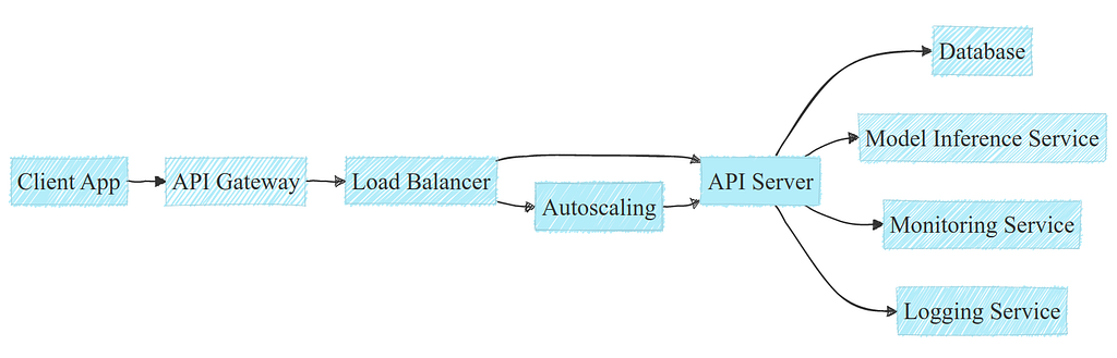
Under the hood, what happens when calling an API might be a bit more complex. API deployments usually involve a standard tech stack including load balancers, autoscalers and interactions with a database:
A typical example of an API deployment within a cloud infrastructure. Image by author.
Note: APIs may have different needs and infrastructure, this example is simplified for clarity.
API deployments are popular for several reasons:
Easy to implement and to integrate into various tech stacks
It’s easy to scale: using horizontal scaling in clouds allow to scale efficiently; moreover managed services of cloud providers may reduce the need for manual intervention
It allows centralized management of model versions and logging, thus efficient tracking and reproducibility
While APIs are a really popular option, there are some cons too:
There might be latency challenges with potential network overhead or geographical distance; and of course it requires a good internet connection
The cost can climb up pretty quickly with high traffic (assuming automatic scaling)
Maintenance overhead can get expensive, either with managed services cost of infra team
To sum up, API deployment is largely used in many startups and tech companies because of its flexibility and a rather short time to market. But the cost can climb up quite fast for high traffic, and the maintenance cost can also be significant.
About the tech stack: there are many ways to develop APIs, but the most common ones in Machine Learning are probably FastAPI and Flask. They can then be deployed quite easily on the main cloud providers (AWS, GCP, Azure…), preferably through docker images. The orchestration can be done through managed services or with Kubernetes, depending on the team’s choice, its size, and skills.
As an example of API cloud deployment, I once deployed a ML solution to automate the pricing of an electric vehicle charging station for a customer-facing web app. You can have a look at this project here if you want to know more about it:
Even if this post does not get into the code, it can give you a good idea of what can be done with API deployment.
API deployment is very popular for its simplicity to integrate to any project. But some projects may need even more flexibility and less maintenance cost: this is where serverless deployment may be a solution.
Serverless Deployment
Another popular, but probably less frequently used option is serverless deployment. Serverless computing means that you run your model (or any code actually) without owning nor provisioning any server.
Serverless deployment offers several significant advantages and is quite easy to set up:
No need to manage nor to maintain servers
No need to handle scaling in case of higher traffic
You only pay for what you use: no traffic means virtually no cost, so no overhead cost at all
But it has some limitations as well:
It is usually not cost effective for large number of queries compared to managed APIs
Cold start latency is a potential issue, as a server might need to be spawned, leading to delays
The memory footprint is usually limited by design: you can’t always run large models
The execution time is limited too: it’s not possible to run jobs for more than a few minutes (15 minutes for AWS Lambda for example)
In a nutshell, I would say that serverless deployment is a good option when you’re launching something new, don’t expect large traffic and don’t want to spend much on infra management.
I personally have never deployed a serverless solution (working mostly with deep learning, I usually found myself limited by the serverless constraints mentioned above), but there is lots of documentation about how to do it properly, such as this one from AWS.
While serverless deployment offers a flexible, on-demand solution, some applications may require a more scheduled approach, like batch processing.
Batch Processing
Another way to deploy on the cloud is through scheduled batch processing. While serverless and APIs are mostly used for live predictions, in some cases batch predictions makes more sense.
Whether it be database updates, dashboard updates, caching predictions… as soon as there is no need to have a real-time prediction, batch processing is usually the best option:
Processing large batches of data is more resource-efficient and reduce overhead compared to live processing
Processing can be scheduled during off-peak hours, allowing to reduce the overall charge and thus the cost
Of course, it comes with associated drawbacks:
Batch processing creates a spike in resource usage, which can lead to system overload if not properly planned
Handling errors is critical in batch processing, as you need to process a full batch gracefully at once
Batch processing should be considered for any task that does not required real-time results: it is usually more cost effective. But of course, for any real-time application, it is not a viable option.
It is used widely in many companies, mostly within ETL (Extract, Transform, Load) pipelines that may or may not contain ML. Some of the most popular tools are:
Apache Airflow for workflow orchestration and task scheduling
Apache Spark for fast, massive data processing
As an example of batch processing, I used to work on a YouTube video revenue forecasting. Based on the first data points of the video revenue, we would forecast the revenue over up to 5 years, using a multi-target regression and curve fitting:
Plot representing the initial data, multi-target regression predictions and curve fitting. Image by author.
For this project, we had to re-forecast on a monthly basis all our data to ensure there was no drifting between our initial forecasting and the most recent ones. For that, we used a managed Airflow, so that every month it would automatically trigger a new forecasting based on the most recent data, and store those into our databases. If you want to know more about this project, you can have a look at this article:
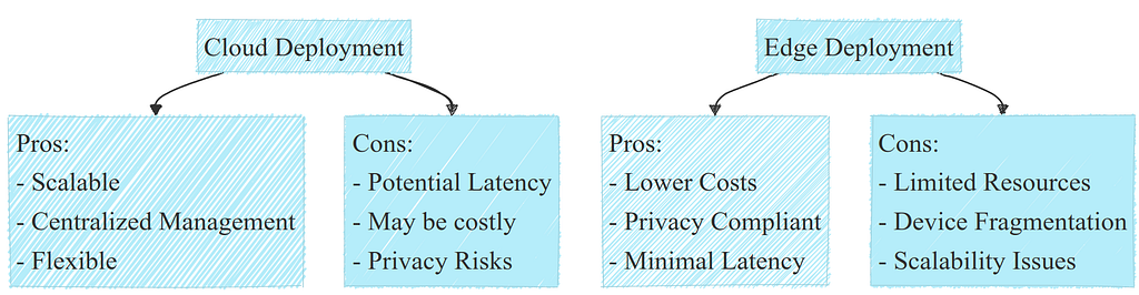
After exploring the various strategies and tools available for cloud deployment, it’s clear that this approach offers significant flexibility and scalability. However, cloud deployment is not always the best fit for every ML application, particularly when real-time processing, privacy concerns, or financial resource constraints come into play.
A list of pros and cons for cloud deployment. Image by author.
This is where edge deployment comes into focus as a viable option. Let’s now delve into edge deployment to understand when it might be the best option.
Edge Deployment
From my own experience, edge deployment is rarely considered as the main way of deployment. A few years ago, even I thought it was not really an interesting option for deployment. With more perspective and experience now, I think it must be considered as the first option for deployment anytime you can.
Just like cloud deployment, edge deployment covers a wide range of cases:
Native phone applications
Web applications
Edge server and specific devices
While they all share some similar properties, such as limited resources and horizontal scaling limitations, each deployment choice may have their own characteristics. Let’s have a look.
Native Application
We see more and more smartphone apps with integrated AI nowadays, and it will probably keep growing even more in the future. While some Big Tech companies such as OpenAI or Google have chosen the API deployment approach for their LLMs, Apple is currently working on the iOS app deployment model with solutions such as OpenELM, a tini LLM. Indeed, this option has several advantages:
The infra cost if virtually zero: no cloud to maintain, it all runs on the device
Better privacy: you don’t have to send any data to an API, it can all run locally
Your model is directly integrated to your app, no need to maintain several codebases
Moreover, Apple has built a fantastic ecosystem for model deployment in iOS: you can run very efficiently ML models with Core ML on their Apple chips (M1, M2, etc…) and take advantage of the neural engine for really fast inferences. To my knowledge, Android is slightly lagging behind, but also has a great ecosystem.
While this can be a really beneficial approach in many cases, there are still some limitations:
Phone resources limit model size and performance, and are shared with other apps
Heavy models may drain the battery pretty fast, which can be deceptive for the user experience overall
Device fragmentation, as well as iOS and Android apps make it hard to cover the whole market
Decentralized model updates can be challenging compared to cloud
Despite its drawbacks, native app deployment is often a strong choice for ML solutions that run in an app. It may seem more complex during the development phase, but it will turn out to be much cheaper as soon as it’s deployed compared to a cloud deployment.
When it comes to the tech stack, there are actually two main ways to deploy: iOS and Android. They both have their own stacks, but they share the same properties:
App development: Swift for iOS, Kotlin for Android
Model format: Core ML for iOS, TensorFlow Lite for Android
Hardware accelerator: Apple Neural Engine for iOS, Neural Network API for Android
Note: This is a mere simplification of the tech stack. This non-exhaustive overview only aims to cover the essentials and let you dig in from there if interested.
As a personal example of such deployment, I once worked on a book reading app for Android, in which they wanted to let the user navigate through the book with phone movements. For example, shake left to go to the previous page, shake right for the next page, and a few more movements for specific commands. For that, I trained a model on accelerometer’s features from the phone for movement recognition with a rather small model. It was then deployed directly in the app as a TensorFlow Lite model.
Native application has strong advantages but is limited to one type of device, and would not work on laptops for example. A web application could overcome those limitations.
Web Application
Web application deployment means running the model on the client side. Basically, it means running the model inference on the device used by that browser, whether it be a tablet, a smartphone or a laptop (and the list goes on…). This kind of deployment can be really convenient:
Your deployment is working on any device that can run a web browser
The inference cost is virtually zero: no server, no infra to maintain… Just the customer’s device
Only one codebase for all possible devices: no need to maintain an iOS app and an Android app simultaneously
Note: Running the model on the server side would be equivalent to one of the cloud deployment options above.
While web deployment offers appealing benefits, it also has significant limitations:
Proper resource utilization, especially GPU inference, can be challenging with TensorFlow.js
Your web app must work with all devices and browsers: whether is has a GPU or not, Safari or Chrome, a Apple M1 chip or not, etc… This can be a heavy burden with a high maintenance cost
You may need a backup plan for slower and older devices: what if the device can’t handle your model because it’s too slow?
Unlike for a native app, there is no official size limitation for a model. However, a small model will be downloaded faster, making it overall experience smoother and must be a priority. And a very large model may just not work at all anyway.
In summary, while web deployment is powerful, it comes with significant limitations and must be used cautiously. One more advantage is that it might be a door to another kind of deployment that I did not mention: WeChat Mini Programs.
The tech stack is usually the same as for web development: HTML, CSS, JavaScript (and any frameworks you want), and of course TensorFlow Lite for model deployment. If you’re curious about an example of how to deploy ML in the browser, you can have a look at this post where I run a real time face recognition model in the browser from scratch:
This article goes from a model training in PyTorch to up to a working web app and might be informative about this specific kind of deployment.
In some cases, native and web apps are not a viable option: we may have no such device, no connectivity, or some other constraints. This is where edge servers and specific devices come into play.
Edge Servers and Specific Devices
Besides native and web apps, edge deployment also includes other cases:
Deployment on edge servers: in some cases, there are local servers running models, such as in some factory production lines, CCTVs, etc…Mostly because of privacy requirements, this solution is sometimes the only available
Deployment on specific device: either a sensor, a microcontroller, a smartwatch, earplugs, autonomous vehicle, etc… may run ML models internally
Deployment on edge servers can be really close to a deployment on cloud with API, and the tech stack may be quite close.
Note: It is also possible to run batch processing on an edge server, as well as just having a monolithic script that does it all.
But deployment on specific devices may involve using FPGAs or low-level languages. This is another, very different skillset, that may differ for each type of device. It is sometimes referred to as TinyML and is a very interesting, growing topic.
On both cases, they share some challenges with other edge deployment methods:
Resources are limited, and horizontal scaling is usually not an option
The battery may be a limitation, as well as the model size and memory footprint
Even with these limitations and challenges, in some cases it’s the only viable solution, or the most cost effective one.
An example of an edge server deployment I did was for a company that wanted to automatically check whether the orders were valid in fast food restaurants. A camera with a top down view would look at the plateau, compare what is sees on it (with computer vision and object detection) with the actual order and raise an alert in case of mismatch. For some reason, the company wanted to make that on edge servers, that were within the fast food restaurant.
To recap, here is a big picture of what are the main types of deployment and their pros and cons:
A list of pros and cons for cloud deployment. Image by author.
With that in mind, how to actually choose the right deployment method? There’s no single answer to that question, but let’s try to give some rules in the next section to make it easier.
How to Choose the Right Deployment
Before jumping to the conclusion, let’s make a decision tree to help you choose the solution that fits your needs.
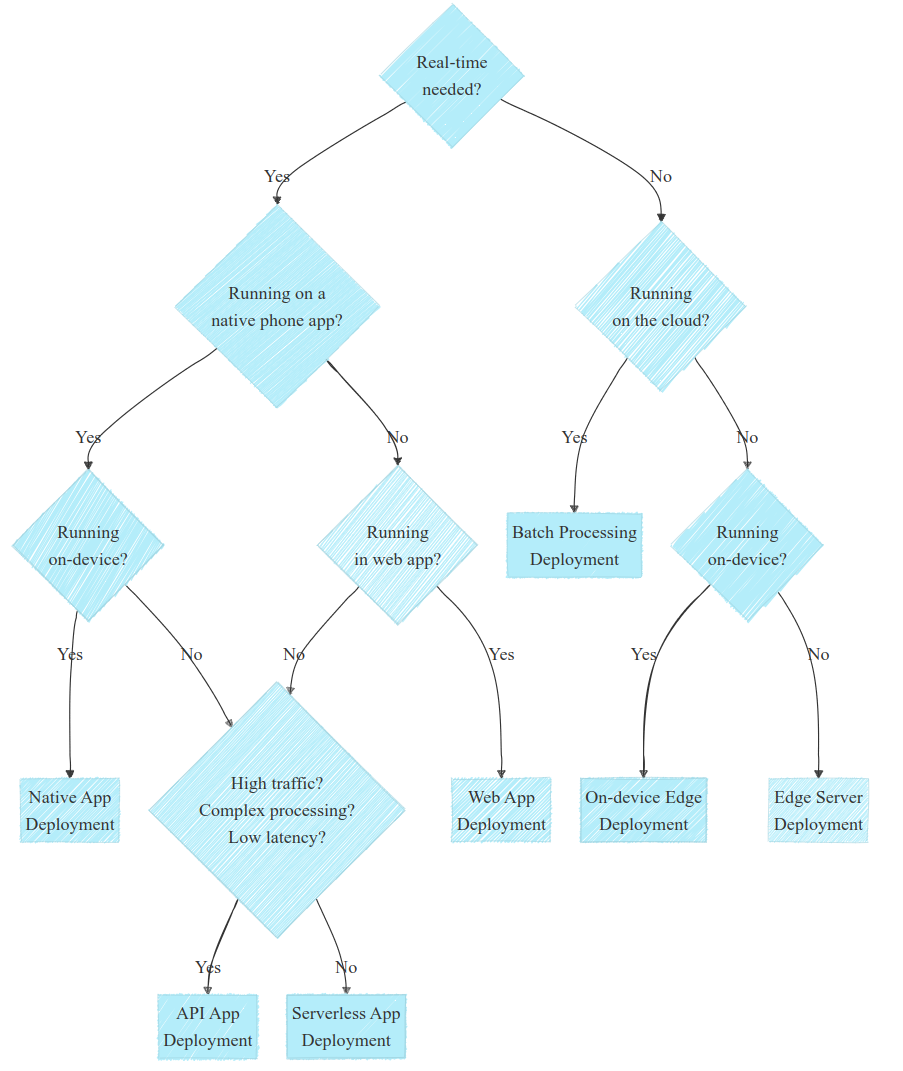
Choosing the right deployment requires understanding specific needs and constraints, often through discussions with stakeholders. Remember that each case is specific and might be a edge case. But in the diagram below I tried to outline the most common cases to help you out:
Deployment decision diagram. Note that each use case is specific. Image by author.
This diagram, while being quite simplistic, can be reduced to a few questions that would allow you go in the right direction:
Do you need real-time? If no, look for batch processing first; if yes, think about edge deployment
Is your solution running on a phone or in the web? Explore these deployments method whenever possible
Is the processing quite complex and heavy? If yes, consider cloud deployment
Again, that’s quite simplistic but helpful in many cases. Also, note that a few questions were omitted for clarity but are actually more than important in some context: Do you have privacy constraints? Do you have connectivity constraints? What is the skillset of your team?
Other questions may arise depending on the use case; with experience and knowledge of your ecosystem, they will come more and more naturally. But hopefully this may help you navigate more easily in deployment of ML models.
Conclusion and Final Thoughts
While cloud deployment is often the default for ML models, edge deployment can offer significant advantages: cost-effectiveness and better privacy control. Despite challenges such as processing power, memory, and energy constraints, I believe edge deployment is a compelling option for many cases. Ultimately, the best deployment strategy aligns with your business goals, resource constraints and specific needs.
If you’ve made it this far, I’d love to hear your thoughts on the deployment approaches you used for your projects.
Discover how LDA helps identify critical data features
Classification of LDA within AI and ML Methods | image by author
This article aims to explore Linear Discriminant Analysis (LDA), focusing on its core ideas, its mathematical implementation in code, and a practical example from manufacturing. I hope you’re on board. Let’s get started!
Who works with industrial data in practice will be familiar with this situation: The datasets usually have many features, and it is often unclear which of the features are important and which are less. “Important” is a relative term in this context. Often, the goal is to differentiate the datasets from each other, i.e., to classify them. A very typical task is to distinguish good parts from bad parts and to identify the causes (aka features) that lead to the failure of the parts.
A commonly used method is the well-known Principal Component Analysis (PCA). While PCA belongs to the unsupervised methods, the less widespread LDA is a supervised method and thus learns from labeled data. Therefore, it is particularly suited for explaining failure patterns from large datasets.
1. Goal and Principle of LDA
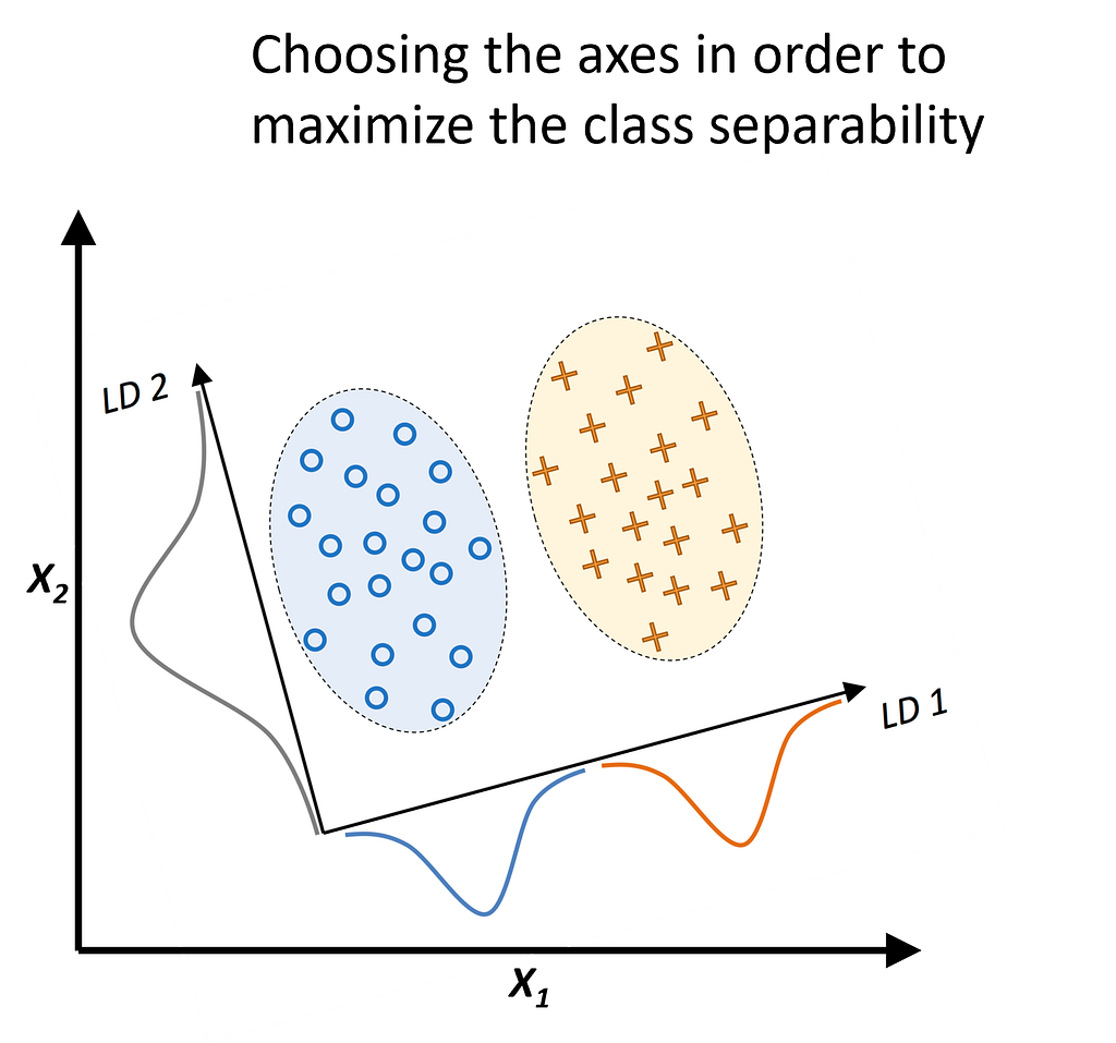
The goal of LDA is to linearly combine the features of the data so that the labels of the datasets are best separated from each other, and the number of new features is reduced to a predefined count. In AI jargon, this is typically referred to as a projection to a lower-dimensional space.
Excursus: What is dimensionality and what is dimensionality reduction?
Dimensions and graphical representation | image by author
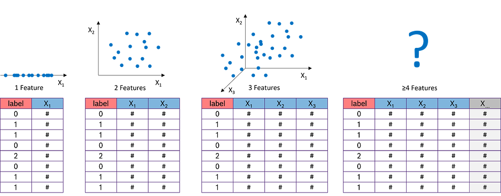
Dimensionality refers to the number of features in a dataset. With just one measurement (or feature), such as the tool temperature from an injection molding machine, we can represent it on a number line. Two features, like temperature and tool pressure, are still manageable: we can easily plot the data on an x-y chart. With three features — temperature, tool pressure, and injection pressure — things get more interesting, but we can still plot the data in a 3D x-y-z chart. However, when we add more features, such as viscosity, electrical conductivity, and others, the complexity increases.
Dimensionality reduction | image by author
In practice, datasets often contain hundreds or even thousands of features. This presents a challenge because many machine learning algorithms perform poorly as datasets grow too large. Additionally, the amount of data required increases exponentially with the number of dimensions to achieve statistical significance. This phenomenon is known as the “curse of dimensionality.” These factors make it essential to determine which features are relevant and to eliminate the less meaningful ones early in the data science process.
2. How does LDA work?
The process of Linear Discriminant Analysis (LDA) can be broken down into five key steps.
Step 1: Compute the d-dimensional mean vectors for each of the k classes separately from the dataset.
Remember that LDA is a supervised machine learning technique, meaning we can utilize the known labels. In the first step, we calculate the mean vectors mean_c for all samples belonging to a specific class c. To do this, we filter the feature matrix by class label and compute the mean for each of the d features. As a result, we obtain k mean vectors (one for each of the k classes), each with a length of d (corresponding to the d features).
Label vector Y and feature matrix X | image by author
Step 2: Compute the scatter matrices (between-class scatter matrix and within-class scatter matrix).
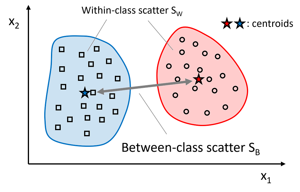
The within-class scatter matrix measures the variation among samples within the same class. To find a subspace with optimal separability, we aim to minimize the values in this matrix. In contrast, the between-class scatter matrix measures the variation between different classes. For optimal separability, we aim to maximize the values in this matrix. Intuitively, within-class scatter looks at how compact each class is, whereas between-class scatter examines how far apart different classes are.
Within-class and between-class scatter matrices | image by author
Let’s start with the within-class scatter matrix S_W. It is calculated as the sum of the scatter matrices S_c for each individual class:
The between-class scatter matrix S_B is derived from the differences between the class means mean_c and the overall mean of the entire dataset:
where mean refers to the mean vector calculated over all samples, regardless of their class labels.
Step 3: Calculate the eigenvectors and eigenvalues for the ratio of S_W and S_B.
As mentioned, for optimal class separability, we aim to maximize S_B and minimize S_W. We can achieve both by maximizing the ratio S_B/S_W. In linear algebra terms, this ratio corresponds to the scatter matrix S_W⁻¹ S_B, which is maximized in the subspace spanned by the eigenvectors with the highest eigenvalues. The eigenvectors define the directions of this subspace, while the eigenvalues represent the magnitude of the distortion. We will select the m eigenvectors associated with the highest eigenvalues.
Subspace spanned by eigenvectors | image by author
Step 4: Sort the eigenvectors in descending order of their corresponding eigenvalues, and select the m eigenvectors with the largest eigenvalues to form a d × m-dimensional transformation matrix W.
Remember, our goal is not only to project the data into a subspace that enhances class separability but also to reduce dimensionality. The eigenvectors will define the axes of our new feature subspace. To decide which eigenvectors to discard for the lower-dimensional subspace, we need to examine their corresponding eigenvalues. In simple terms, the eigenvectors with the smallest eigenvalues contribute the least to class separation, and these are the ones we want to drop. The typical approach is to rank the eigenvalues in descending order and select the top m eigenvectors. m is a freely chosen parameter. The larger m, the less information is lost during the transformation.
After sorting the eigenpairs by decreasing eigenvalues and selecting the top m pairs, the next step is to construct the d × m-dimensional transformation matrix W. This is done by stacking the m selected eigenvectors horizontally, resulting in the matrix W:
The first column of W represents the eigenvector corresponding to the highest eigenvalue, the second column represents the eigenvector corresponding to the second highest eigenvalue, and so on.
Step 5: Use W to project the samples onto the new subspace.
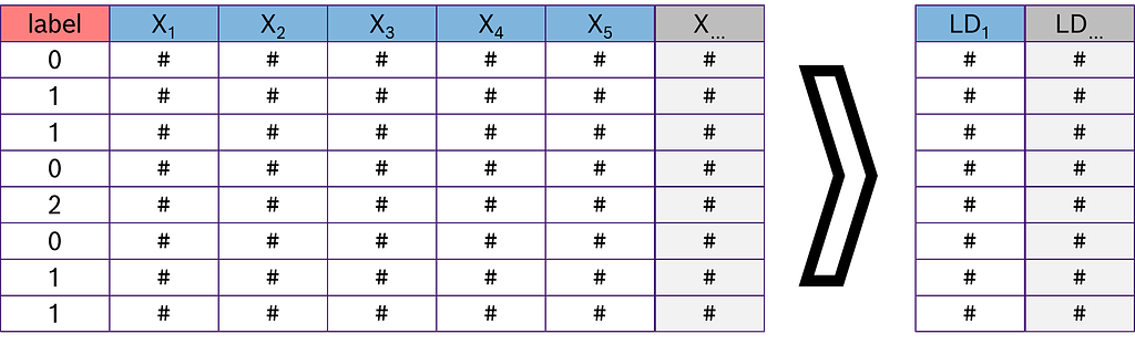
In the final step, we use the d × m-dimensional transformation matrix W, which we composed from the top m selected eigenvectors, to project our samples onto the new subspace:
where X is the initial n × d-dimensional feature matrix representing our samples, and Z is the newly transformed n × m-dimensional feature matrix in the new subspace. This means that the selected eigenvectors serve as the “recipes” for transforming the original features into the new features (the Linear Discriminants): The eigenvector with the highest eigenvalue provides the transformation recipe for LD1, the eigenvector with the second highest eigenvalue corresponds to LD2, and so on.
Projection of X onto the linear discriminants LD
3. Implementing Linear Discriminant Analysis (LDA) from Scratch
To demonstrate the theory and mathematics in action, we will program our own LDA from scratch using only numpy.
import numpy as np


class LDA_fs:
    """
    Performs a Linear Discriminant Analysis (LDA)

    Methods
    =======
    fit_transform():
        Fits the model to the data X and Y, derives the transformation matrix W
    and projects the feature matrix X onto the m LDA axes
    """

    def __init__(self, m):
        """
        Parameters
        ==========
        m : int
            Number of LDA axes onto which the data will be projected

        Returns
        =======
        None
        """
        self.m = m

    def fit_transform(self, X, Y):
        """
        Parameters
        ==========
        X : array(n_samples, n_features)
            Feature matrix of the dataset
        Y = array(n_samples)
            Label vector of the dataset

        Returns
        =======
        X_transform : New feature matrix projected onto the m LDA axes

        """

        # Get number of features (columns)
        self.n_features = X.shape[1]
        # Get unique class labels
        class_labels = np.unique(Y)
        # Get the overall mean vector (independent of the class labels)
        mean_overall = np.mean(X, axis=0)  # Mean of each feature
        # Initialize both scatter matrices with zeros
        SW = np.zeros((self.n_features, self.n_features))  # Within scatter matrix
        SB = np.zeros((self.n_features, self.n_features))  # Between scatter matrix

        # Iterate over all classes and select the corresponding data
        for c in class_labels:
            # Filter X for class c
            X_c = X[Y == c]
            # Calculate the mean vector for class c
            mean_c = np.mean(X_c, axis=0)
            # Calculate within-class scatter for class c
            SW += (X_c - mean_c).T.dot((X_c - mean_c))
            # Number of samples in class c
            n_c = X_c.shape[0]
            # Difference between the overall mean and the mean of class c --> between-class scatter
            mean_diff = (mean_c - mean_overall).reshape(self.n_features, 1)
            SB += n_c * (mean_diff).dot(mean_diff.T)

        # Determine SW^-1 * SB
        A = np.linalg.inv(SW).dot(SB)
        # Get the eigenvalues and eigenvectors of (SW^-1 * SB)
        eigenvalues, eigenvectors = np.linalg.eig(A)
        # Keep only the real parts of eigenvalues and eigenvectors
        eigenvalues = np.real(eigenvalues)
        eigenvectors = np.real(eigenvectors.T)

        # Sort the eigenvalues descending (high to low)
        idxs = np.argsort(np.abs(eigenvalues))[::-1]
        self.eigenvalues = np.abs(eigenvalues[idxs])
        self.eigenvectors = eigenvectors[idxs]
        # Store the first m eigenvectors as transformation matrix W
        self.W = self.eigenvectors[0:self.m]

        # Transform the feature matrix X onto LD axes
        return np.dot(X, self.W.T)
4. Applying LDA to an Industrial Dataset
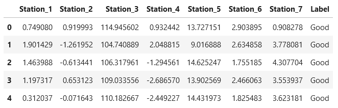
To see LDA in action, we will apply it to a typical task in the production environment. We have data from a simple manufacturing line with only 7 stations. Each of these stations sends a data point (yes, I know, only one data point is highly unrealistic). Unfortunately, our line produces a significant number of defective parts, and we want to find out which stations are responsible for this.
First, we load the data and take an initial look.
import pandas as pd

# URL to Github repository
url = "https://raw.githubusercontent.com/IngoNowitzky/LDA_Medium/main/production_line_data.csv"

# Read csv to DataFrame
data = pd.read_csv(url)

# Print first 5 lines
data.head()
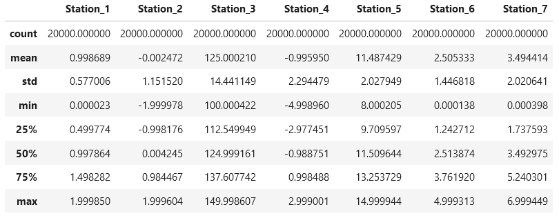
Next, we study the distribution of the data using the .describe() method from Pandas.
# Show average, min and max of numerical values
data.describe()
We see that we have 20,000 data points, and the measurements range from -5 to +150. Hence, we note for later that we need to normalize the dataset: the different magnitudes of the numerical values would otherwise negatively affect the LDA. How many good parts and how many bad parts do we have?
# Count the number of good and bad parts
label_counts = data['Label'].value_counts()

# Display the results
print("Number of Good and Bad Parts:")
print(label_counts)
We have 19,031 good parts and 969 defective parts. The fact that the dataset is so imbalanced is an issue for further analysis. Therefore, we select all defective parts and an equal number of randomly chosen good parts for the further processing.
# Select all bad parts
bad_parts = data[data['Label'] == 'Bad']

# Randomly select an equal number of good parts
good_parts = data[data['Label'] == 'Good'].sample(n=len(bad_parts), random_state=42)

# Combine both subsets to create a balanced dataset
balanced_data = pd.concat([bad_parts, good_parts])

# Shuffle the combined dataset
balanced_data = balanced_data.sample(frac=1, random_state=42).reset_index(drop=True)

# Display the number of good and bad parts in the balanced dataset
print("Number of Good and Bad Parts in the balanced dataset:")
print(balanced_data['Label'].value_counts())
Now, let’s apply our LDA from scratch to the balanced dataset. We use the StandardScaler from sklearn to normalize the measurements for each feature to have a mean of 0 and a standard deviation of 1. We choose only one linear discriminant axis (m=1) onto which we project the data. This helps us clearly see which features are most relevant in distinguishing good from bad parts, and we visualize the projected data in a histogram.
import matplotlib.pyplot as plt
from sklearn.preprocessing import StandardScaler

# Separate features and labels
X = balanced_data.drop(columns=['Label'])
y = balanced_data['Label']

# Normalize the features
scaler = StandardScaler()
X_scaled = scaler.fit_transform(X)

# Perform LDA
lda = LDA_fs(m=1)  # Instanciate LDA object with 1 axis
X_lda = lda.fit_transform(X_scaled, y) # Fit the model and project the data

# Plot the LDA projection
plt.figure(figsize=(10, 6))
plt.hist(X_lda[y == 'Good'], bins=20, alpha=0.7, label='Good', color='green')
plt.hist(X_lda[y == 'Bad'], bins=20, alpha=0.7, label='Bad', color='red')
plt.title("LDA Projection of Good and Bad Parts")
plt.xlabel("LDA Component")
plt.ylabel("Frequency")
plt.legend()
plt.show()

# Examine feature contributions to the LDA component
feature_importance = pd.DataFrame({'Feature': X.columns, 'LDA Coefficient': lda.W[0]})
feature_importance = feature_importance.sort_values(by='LDA Coefficient', ascending=False)

# Display feature importance
print("Feature Contributions to LDA Component:")
print(feature_importance)
Feature matrix projected to one LD (m=1)Feature importance = How much do the stations contribute to class separation?
The histogram shows that we can separate the good parts from the defective parts very well, with only a small overlap. This is already a positive result and indicates that our LDA was successful.
The “LDA Coefficients” from the table “Feature Contributions to LDA Components” represent the eigenvector from the first (and only, since m=1) column of our transformation matrix W. They indicate the direction and magnitude with which the normalized measurements from the stations are projected onto the linear discriminant axis. The values in the table are sorted in descending order. We need to read the table from both the top and the bottom simultaneously because the absolute value of the coefficient indicates the significance of each station in separating the classes and, consequently, its contribution to the production of defective parts. The sign indicates whether a lower or higher measurement increases the likelihood of defective parts. Let’s take a closer look at our example:
The largest absolute value is from Station 4, with a coefficient of -0.672. This means that Station 4 has the strongest influence on part failure. Due to the negative sign, higher positive measurements are projected towards a negative linear discriminant (LD). The histogram shows that a negative LD is associated with good (green) parts. Conversely, low and negative measurements at this station increase the likelihood of part failure. The second highest absolute value is from Station 2, with a coefficient of 0.557. Therefore, this station is the second most significant contributor to part failures. The positive sign indicates that high positive measurements are projected towards the positive LD. From the histogram, we know that a high positive LD value is associated with a high likelihood of failure. In other words, high measurements at Station 2 lead to part failures. The third highest coefficient comes from Station 7, with a value of -0.486. This makes Station 7 the third largest contributor to part failures. The negative sign again indicates that high positive values at this station lead to a negative LD (which corresponds to good parts). Conversely, low and negative values at this station lead to part failures. All other LDA coefficients are an order of magnitude smaller than the three mentioned, the associated stations therefore have no influence on part failure.
Are the results of our LDA analysis correct? As you may have already guessed, the production dataset is synthetically generated. I labeled all parts as defective where the measurement at Station 2 was greater than 0.5, the value at Station 4 was less than -2.5, and the value at Station 7 was less than 3. It turns out that the LDA hit the mark perfectly!
# Determine if a sample is a good or bad part based on the conditions
data['Label'] = np.where(
    (data['Station_2'] > 0.5) & (data['Station_4'] < -2.5) & (data['Station_7'] < 3),
    'Bad',
    'Good'
)
5. Conclusion
Linear Discriminant Analysis (LDA) not only reduces the complexity of datasets but also highlights the key features that drive class separation, making it highly effective for identifying failure causes in production systems. It is a straightforward yet powerful method with practical applications and is readily available in libraries like scikit-learn.
To achieve optimal results, it is crucial to balance the dataset (ensure a similar number of samples in each class) and normalize it (mean of 0 and standard deviation of 1). The next time you work with a large dataset containing class labels and numerous features, why not give LDA a try?
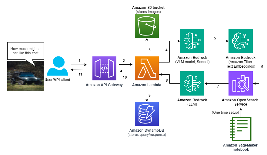
In this post, we show how to create a multimodal chat assistant on Amazon Web Services (AWS) using Amazon Bedrock models, where users can submit images and questions, and text responses will be sourced from a closed set of proprietary documents.
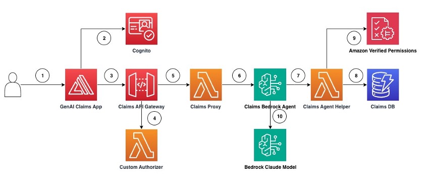
In this post, we demonstrate how to design fine-grained access controls using Verified Permissions for a generative AI application that uses Amazon Bedrock Agents to answer questions about insurance claims that exist in a claims review system using textual prompts as inputs and outputs.
Early holiday deals are now widely available in October, and eBay is no exception with its latest coupon. Save on thousands of items, including Apple hardware, with a huge max discount of up to $500 off.
Get a jumpstart on holiday shopping with this coupon. [eBay]
For less than a week, shoppers can take advantage of 20% off select purchases on eBay.com with promo code SHOPGIFTSEARLY. With the discount capped at a very high $500 off, it’s a great way to save on already reduced prices, with thousands of gift ideas to choose from.
A Monday price war on Apple’s M4 iPad Pro has developed at Amazon and B&H, with 11-inch and 13-inch models up to $207 off. Plus, grab the lowest price in 30 days on the Apple Pencil Pro.
Save on Apple’s M4 iPad Pro line.
We’re keeping tabs on the best iPad deals this October and today’s top offers include markdowns on Apple’s latest iPad Pro, along with a fresh price drop on the complementary Apple Pencil Pro.
Pick up the standard 2024 11-inch iPad Pro this Monday for just $899, a discount of $100 off retail. This Standard Glass spec with 256GB capacity and Wi-Fi connectivity is eligible for the reduced price at both Amazon and B&H Photo in your choice of Space Black or Silver.
We use cookies on our website to give you the most relevant experience by remembering your preferences and repeat visits. By clicking “Accept”, you consent to the use of ALL the cookies.
This website uses cookies to improve your experience while you navigate through the website. Out of these, the cookies that are categorized as necessary are stored on your browser as they are essential for the working of basic functionalities of the website. We also use third-party cookies that help us analyze and understand how you use this website. These cookies will be stored in your browser only with your consent. You also have the option to opt-out of these cookies. But opting out of some of these cookies may affect your browsing experience.
Necessary cookies are absolutely essential for the website to function properly. These cookies ensure basic functionalities and security features of the website, anonymously.
Cookie
Duration
Description
cookielawinfo-checkbox-analytics
11 months
This cookie is set by GDPR Cookie Consent plugin. The cookie is used to store the user consent for the cookies in the category "Analytics".
cookielawinfo-checkbox-functional
11 months
The cookie is set by GDPR cookie consent to record the user consent for the cookies in the category "Functional".
cookielawinfo-checkbox-necessary
11 months
This cookie is set by GDPR Cookie Consent plugin. The cookies is used to store the user consent for the cookies in the category "Necessary".
cookielawinfo-checkbox-others
11 months
This cookie is set by GDPR Cookie Consent plugin. The cookie is used to store the user consent for the cookies in the category "Other.
cookielawinfo-checkbox-performance
11 months
This cookie is set by GDPR Cookie Consent plugin. The cookie is used to store the user consent for the cookies in the category "Performance".
viewed_cookie_policy
11 months
The cookie is set by the GDPR Cookie Consent plugin and is used to store whether or not user has consented to the use of cookies. It does not store any personal data.
Functional cookies help to perform certain functionalities like sharing the content of the website on social media platforms, collect feedbacks, and other third-party features.
Performance cookies are used to understand and analyze the key performance indexes of the website which helps in delivering a better user experience for the visitors.
Analytical cookies are used to understand how visitors interact with the website. These cookies help provide information on metrics the number of visitors, bounce rate, traffic source, etc.
Advertisement cookies are used to provide visitors with relevant ads and marketing campaigns. These cookies track visitors across websites and collect information to provide customized ads.


