Ethereum lagged behind Bitcoin with a weaker 2024 performance and tepid ETF demand
Experts and traders feel differently about Ethereum’s future, with opinions ranging from bullish to cautious
Altcoin recently broke out of a descending channel, indicating the start of a potential upswing
Large-volume traders are yet to enter the market, leaving retail investors to drive the price act
UNI’s charts flashed strong bullish momentum after breaking out of a descending channel with rising volume
Positive on-chain metrics and falling exchange reserves could serve altcoin well
Cardano, the industry’s ninth-largest crypto by market cap has started 2025 on a roll, zooming past the $1 price milestone for the first time since Dec. 18, 2024.
The crypto market is witnessing significant developments, with Toncoin (TON), Avalanche (AVAX), and BlockDAG (BDAG) leading the game. Recent Toncoin price predictions suggest that, after a 140% surge in 2024, TON could reach $16.65 this year. Similarly, AVAX price trends show promise, pointing to a potential rise to $81 in 2025, driven by strong DeFi […]
Full explanation on Linear Regression and how it learns
The Crane Stance. Public Domain image from Openverse
Just like Mr. Miyagi taught young Daniel LaRusso karate through repetitive simple chores, which ultimately transformed him into the Karate Kid, mastering foundational algorithms like linear regression lays the groundwork for understanding the most complex of AI architectures such as Deep Neural Networks and LLMs.
Through this deep dive into the simple yet powerful linear regression, you will learn many of the fundamental parts that make up the most advanced models built today by billion-dollar companies.
What is Linear Regression?
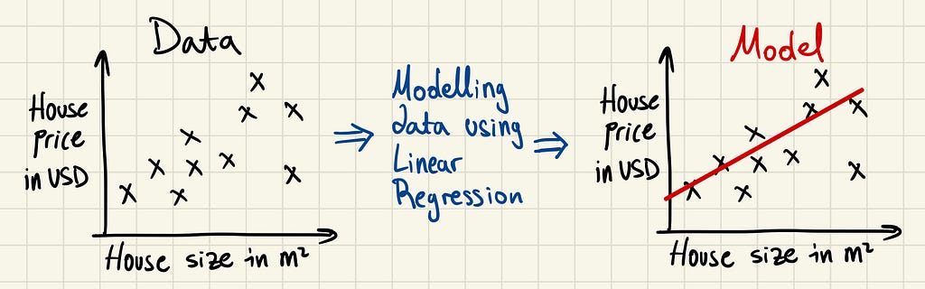
Linear regression is a simple mathematical method used to understand the relationship between two variables and make predictions. Given some data points, such as the one below, linear regression attempts to draw the line of best fit through these points. It’s the “wax on, wax off” of data science.
Example of linear regression model on a graph. Image captured by Author
Once this line is drawn, we have a model that we can use to predict new values. In the above example, given a new house size, we could attempt to predict its price with the linear regression model.
The Linear Regression Formula
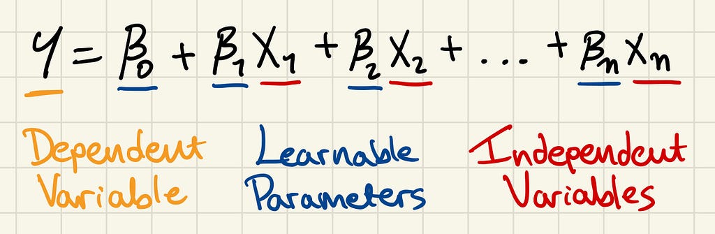
Labelled Linear Regression Formula. Image captured by Author
Y is the dependent variable, that which you want to calculate — the house price in the previous example. Its value depends on other variables, hence its name.
X are the independent variables. These are the factors that influence the value of Y. When modelling, the independent variables are the input to the model, and what the model spits out is the prediction or Ŷ.
β are parameters. We give the name parameter to those values that the model adjusts (or learns) to capture the relationship between the independent variables X and the dependent variable Y. So, as the model is trained, the input of the model will remain the same, but the parameters will be adjusted to better predict the desired output.
Parameter Learning
We require a few things to be able to adjust the parameters and achieve accurate predictions.
Training Data — this data consists of input and output pairs. The inputs will be fed into the model and during training, the parameters will be adjusted in an attempt to output the target value.
Cost function — also known as the loss function, is a mathematical function that measures how well a model’s prediction matches the target value.
Training Algorithm — is a method used to adjust the parameters of the model to minimise the error as measured by the cost function.
Let’s go over a cost function and training algorithm that can be used in linear regression.
Cost Function: Mean Squared Error (MSE)
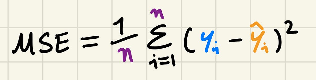
MSE is a commonly used cost function in regression problems, where the goal is to predict a continuous value. This is different from classification tasks, such as predicting the next token in a vocabulary, as in Large Language Models. MSE focuses on numerical differences and is used in a variety of regression and neural network problems, this is how you calculate it:
Mean Squared Error (MSE) formula. Image captured by Author
Calculate the difference between the predicted value, Ŷ, and the target value, Y.
Square this difference — ensuring all errors are positive and also penalising large errors more heavily.
Sum the squared differences for all data samples
Divide the sum by the number of samples, n, to get the average squared error
You will notice that as our prediction gets closer to the target value the MSE gets lower, and the further away they are the larger it grows. Both ways progress quadratically because the difference is squared.
Training Algorithm: Gradient Descent
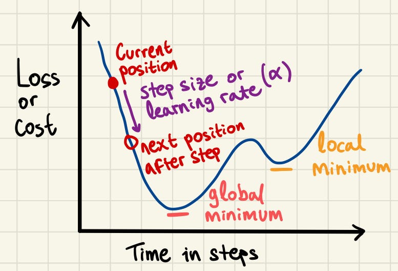
The concept of gradient descent is that we can travel through the “cost space” in small steps, with the objective of arriving at the global minimum — the lowest value in the space. The cost function evaluates how well the current model parameters predict the target by giving us the loss value. Randomly modifying the parameters does not guarantee any improvements. But, if we examine the gradient of the loss function with respect to each parameter, i.e. the direction of the loss after an update of the parameter, we can adjust the parameters to move towards a lower loss, indicating that our predictions are getting closer to the target values.
Labelled graph showing the key concepts of the gradient descent algorithm. Image captured by Author
The steps in gradient descent must be carefully sized to balance progress and precision. If the steps are too large, we risk overshooting the global minimum and missing it entirely. On the other hand, if the steps are too small, the updates will become inefficient and time-consuming, increasing the likelihood of getting stuck in a local minimum instead of reaching the desired global minimum.
Gradient Descent Formula
Labelled Gradient Descent formula. Image captured by Author
In the context of linear regression, θ could be β0 or β1. The gradient is the partial derivative of the cost function with respect to θ, or in simpler terms, it is a measure of how much the cost function changes when the parameter θ is slightly adjusted.
A large gradient indicates that the parameter has a significant effect on the cost function, while a small gradient suggests a minor effect. The sign of the gradient indicates the direction of change for the cost function. A negative gradient means the cost function will decrease as the parameter increases, while a positive gradient means it will increase.
So, in the case of a large negative gradient, what happens to the parameter? Well, the negative sign in front of the learning rate will cancel with the negative sign of the gradient, resulting in an addition to the parameter. And since the gradient is large we will be adding a large number to it. So, the parameter is adjusted substantially reflecting its greater influence on reducing the cost function.
Practical Example
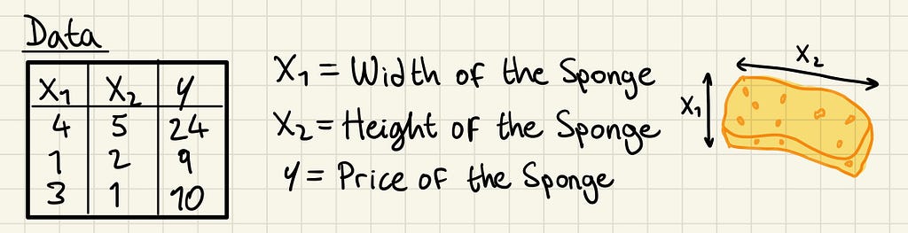
Let’s take a look at the prices of the sponges Karate Kid used to wash Mr. Miyagi’s car. If we wanted to predict their price (dependent variable) based on their height and width (independent variables), we could model it using linear regression.
We can start with these three training data samples.
Training data for the linear regression example modelling prices of sponges. Image captured by Author
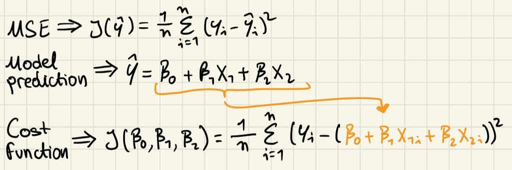
Now, let’s use the Mean Square Error (MSE) as our cost function J, and linear regression as our model.
Formula for the cost function derived from MSE and linear regression. Image captured by Author
The linear regression formula uses X1 and X2 for width and height respectively, notice there are no more independent variables since our training data doesn’t include more. That is the assumption we take in this example, that the width and height of the sponge are enough to predict its price.
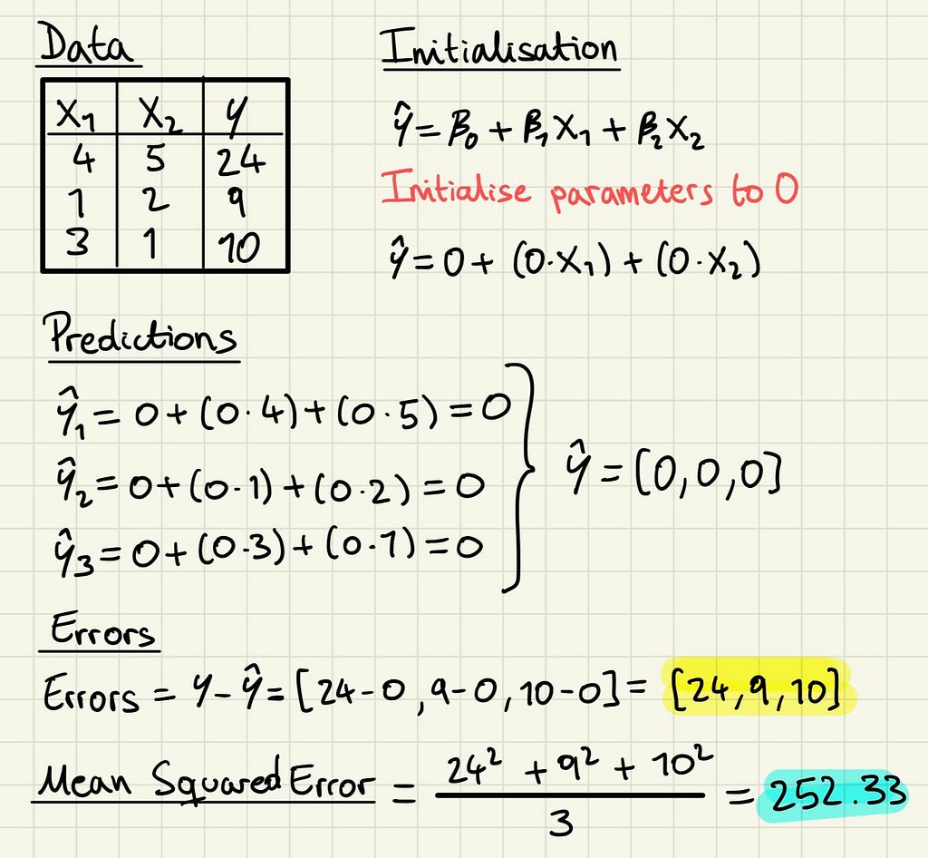
Now, the first step is to initialise the parameters, in this case to 0. We can then feed the independent variables into the model to get our predictions, Ŷ, and check how far these are from our target Y.
Step 0 in gradient descent algorithm and the calculation of the mean squared error. Image captured by Author
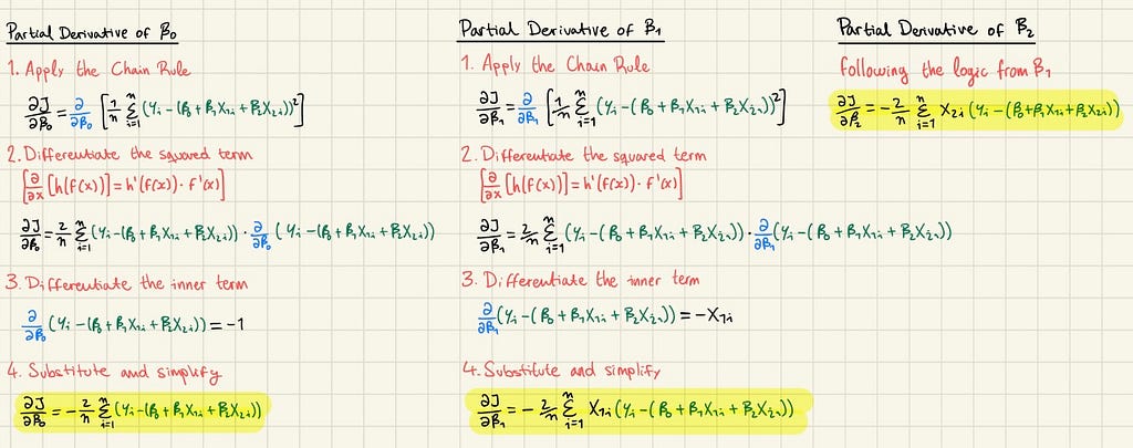
Right now, as you can imagine, the parameters are not very helpful. But we are now prepared to use the Gradient Descent algorithm to update the parameters into more useful ones. First, we need to calculate the partial derivatives of each parameter, which will require some calculus, but luckily we only need to this once in the whole process.
Working out of the partial derivatives of the linear regression parameters. Image captured by Author
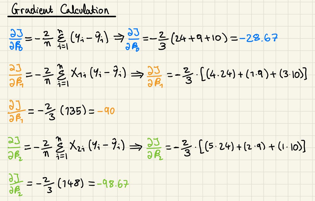
With the partial derivatives, we can substitute in the values from our errors to calculate the gradient of each parameter.
Calculation of parameter gradients. Image captured by Author
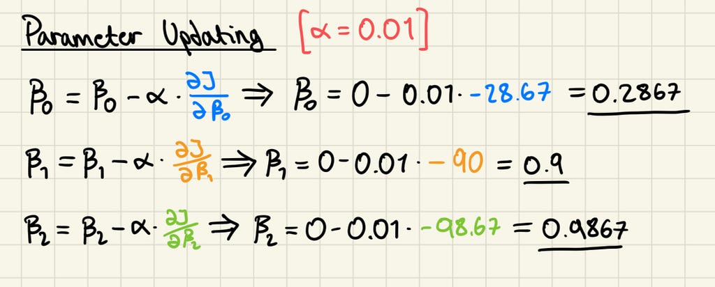
Notice there wasn’t any need to calculate the MSE, as it’s not directly used in the process of updating parameters, only its derivative is. It’s also immediately apparent that all gradients are negative, meaning that all can be increased to reduce the cost function. The next step is to update the parameters with a learning rate, which is a hyper-parameter, i.e. a configuration setting in a machine learning model that is specified before the training process begins. Unlike model parameters, which are learned during training, hyper-parameters are set manually and control aspects of the learning process. Here we arbitrarily use 0.01.
Parameter updating in the first iteration of gradient descent. Image captured by Author
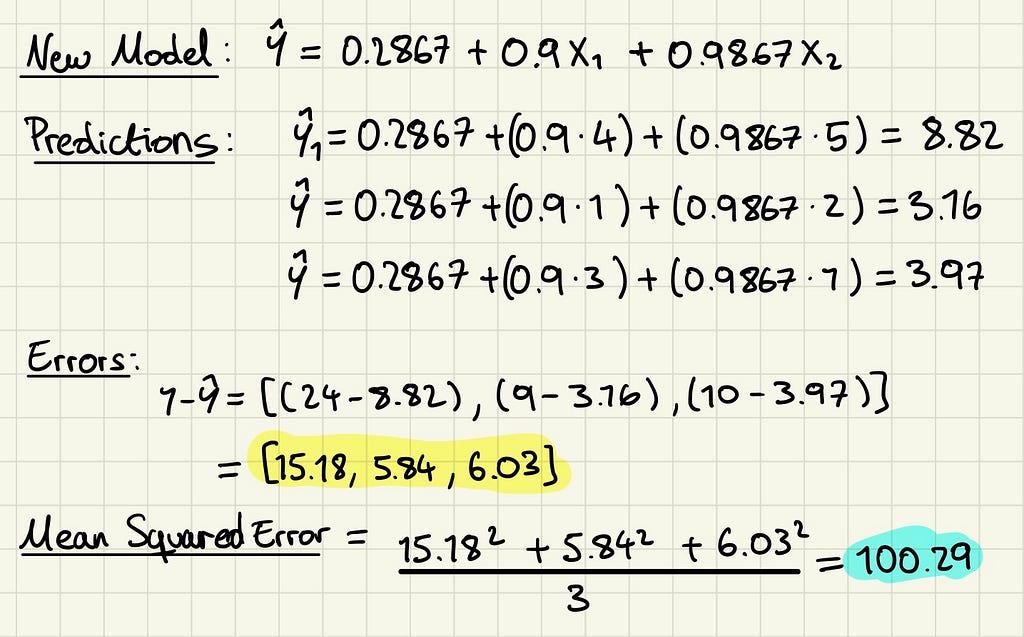
This has been the final step of our first iteration in the process of gradient descent. We can use these new parameter values to make new predictions and recalculate the MSE of our model.
Last step in the first iteration of gradient descent, and recalculation of MSE after parameter updates. Image captured by Author
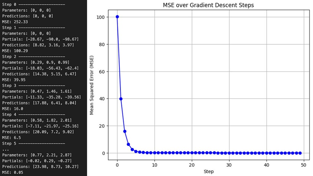
The new parameters are getting closer to the true sponge prices, and have yielded a much lower MSE, but there is a lot more training left to do. If we iterate through the gradient descent algorithm 50 times, this time using Python instead of doing it by hand — since Mr. Miyagi never said anything about coding — we will reach the following values.
Results of some iterations of the gradient descent algorithm, and a graph showing the MSE over the gradient descent steps. Image captured by Author
Eventually we arrived to a pretty good model. The true values I used to generate those numbers were [1, 2, 3] and after only 50 iterations, the model’s parameters came impressively close. Extending the training to 200 steps, which is another hyper-parameter, with the same learning rate allowed the linear regression model to converge almost perfectly to the true parameters, demonstrating the power of gradient descent.
Conclusions
Many of the fundamental concepts that make up the complicated martial art of artificial intelligence, like cost functions and gradient descent, can be thoroughly understood just by studying the simple “wax on, wax off” tool that linear regression is.
Artificial intelligence is a vast and complex field, built upon many ideas and methods. While there’s much more to explore, mastering these fundamentals is a significant first step. Hopefully, this article has brought you closer to that goal, one “wax on, wax off” at a time.
We use cookies on our website to give you the most relevant experience by remembering your preferences and repeat visits. By clicking “Accept”, you consent to the use of ALL the cookies.
This website uses cookies to improve your experience while you navigate through the website. Out of these, the cookies that are categorized as necessary are stored on your browser as they are essential for the working of basic functionalities of the website. We also use third-party cookies that help us analyze and understand how you use this website. These cookies will be stored in your browser only with your consent. You also have the option to opt-out of these cookies. But opting out of some of these cookies may affect your browsing experience.
Necessary cookies are absolutely essential for the website to function properly. These cookies ensure basic functionalities and security features of the website, anonymously.
Cookie
Duration
Description
cookielawinfo-checkbox-analytics
11 months
This cookie is set by GDPR Cookie Consent plugin. The cookie is used to store the user consent for the cookies in the category "Analytics".
cookielawinfo-checkbox-functional
11 months
The cookie is set by GDPR cookie consent to record the user consent for the cookies in the category "Functional".
cookielawinfo-checkbox-necessary
11 months
This cookie is set by GDPR Cookie Consent plugin. The cookies is used to store the user consent for the cookies in the category "Necessary".
cookielawinfo-checkbox-others
11 months
This cookie is set by GDPR Cookie Consent plugin. The cookie is used to store the user consent for the cookies in the category "Other.
cookielawinfo-checkbox-performance
11 months
This cookie is set by GDPR Cookie Consent plugin. The cookie is used to store the user consent for the cookies in the category "Performance".
viewed_cookie_policy
11 months
The cookie is set by the GDPR Cookie Consent plugin and is used to store whether or not user has consented to the use of cookies. It does not store any personal data.
Functional cookies help to perform certain functionalities like sharing the content of the website on social media platforms, collect feedbacks, and other third-party features.
Performance cookies are used to understand and analyze the key performance indexes of the website which helps in delivering a better user experience for the visitors.
Analytical cookies are used to understand how visitors interact with the website. These cookies help provide information on metrics the number of visitors, bounce rate, traffic source, etc.
Advertisement cookies are used to provide visitors with relevant ads and marketing campaigns. These cookies track visitors across websites and collect information to provide customized ads.