Blog

  • How Long Does It Take to Train the LLM From Scratch?

    Max Shap

    Guide to estimating time for training X-billion LLMs with Y trillion tokens and Z GPU compute

    Image by author

    Intro

    Every ML engineer working on LLM training has faced the question from a manager or product owner: ‘How long will it take to train this LLM?’

    When I first tried to find an answer online, I was met with many articles covering generic topics — training techniques, model evaluation, and the like. But none of them addressed the core question I had: How do I actually estimate the time required for training?

    Frustrated by the lack of clear, practical guidance, I decided to create my own. In this article, I’ll walk you through a simple, back-of-the-envelope method to quickly estimate how long it will take to train your LLM based on its size, data volume, and available GPU power

    Approach

    The goal is to quantify the computational requirements for processing data and updating model parameters during training in terms of FLOPs (floating point operations). Next, we estimate the system’s throughput in FLOPS (floating-point operations per second) based on the type and number of GPUs selected. Once everything is expressed on the same scale, we can easily calculate the time required to train the model.

    So the final formula is pretty straightforward:

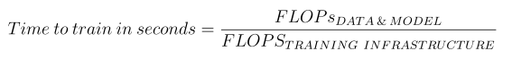
    Let’s dive into knowing how to estimate all these variables.

    FLOPs for Data and Model

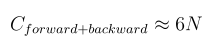
    The number of add-multiply operations per token for the forward pass for Transformer based LLM involves roughly the following amount of FLOPs:

    Approximation of FLOPs per token for the Transformer model of size N during forward pass from paper

    Where the factor of two comes from the multiply-accumulate operation used in matrix multiplication.

    The backward pass requires approximately twice the compute of the forward pass. This is because, during backpropagation, we need to compute gradients for each weight in the model as well as gradients with respect to the intermediate activations, specifically the activations of each layer.

    With this in mind, the floating-point operations per training token can be estimated as:

    Approximation of FLOPs per token for the Transformer model of size N during forward and backward pass from paper

    A more detailed math for deriving these estimates can be found in the paper from the authors here.

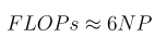
    To sum up, training FLOPs for the transformer model of size N and dataset of P tokens can be estimated as:

    FLOPS of the training Infrastructure

    Today, most LLMs are trained using GPU accelerators. Each GPU model (like Nvidia’s H100, A100, or V100) has its own FLOPS performance, which varies depending on the data type (form factor) being used. For instance, operations with FP64 are slower than those with FP32, and so on. The peak theoretical FLOPS for a specific GPU can usually be found on its product specification page (e.g., here for the H100).

    However, the theoretical maximum FLOPS for a GPU is often less relevant in practice when training Large Language Models. That’s because these models are typically trained on thousands of interconnected GPUs, where the efficiency of network communication becomes crucial. If communication between devices becomes a bottleneck, it can drastically reduce the overall speed, making the system’s actual FLOPS much lower than expected.

    To address this, it’s important to track a metric called model FLOPS utilization (MFU) — the ratio of the observed throughput to the theoretical maximum throughput, assuming the hardware is operating at peak efficiency with no memory or communication overhead. In practice, as the number of GPUs involved in training increases, MFU tends to decrease. Achieving an MFU above 50% is challenging with current setups.

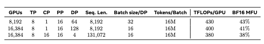
    For example, the authors of the LLaMA 3 paper reported an MFU of 38%, or 380 teraflops of throughput per GPU, when training with 16,000 GPUs.

    Reported TFLOPs throughput per GPU training Llama3 models as reported in the paper for different configurations

    To summarize, when performing a back-of-the-envelope calculation for model training, follow these steps:

    1. Identify the theoretical peak FLOPS for the data type your chosen GPU supports.
    2. Estimate the MFU (model FLOPS utilization) based on the number of GPUs and network topology, either through benchmarking or by referencing open-source data, such as reports from Meta engineers (as shown in the table above).
    3. Multiply the theoretical FLOPS by the MFU to get the average throughput per GPU.
    4. Multiply the result from step 3 by the total number of GPUs involved in training.

    Case study with Llama 3 405B

    Now, let’s put our back-of-the-envelope calculations to work and estimate how long it takes to train a 405B parameter model.

    LLaMA 3.1 (405B) was trained on 15.6 trillion tokens — a massive dataset. The total FLOPs required to train a model of this size can be calculated as follows:

    The authors used 16,000 H100 GPUs for training. According to the paper, the average throughput was 400 teraflops per GPU. This means the training infrastructure can deliver a total throughput of:

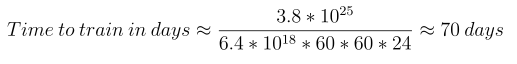
    Finally, by dividing the total required FLOPs by the available throughput and converting the result into days (since what we really care about is the number of training days), we get:

    Bonus: How much does it cost to train Llama 3.1 405B?

    Once you know the FLOPS per GPU in the training setup, you can calculate the total GPU hours required to train a model of a given size and dataset. You can then multiply this number by the cost per GPU hour from your cloud provider (or your own cost per GPU hour).

    For example, if one H100 GPU costs approximately $2 per hour, the total cost to train this model would be around $52 million! The formula below explains how this number is derived:

    References

    [1] Scaling Laws for Neural Language Models by Jared Kaplan et al.

    [2]The Llama 3 Herd of Models by Llama Team, AI @ Meta


    How Long Does It Take to Train the LLM From Scratch? was originally published in Towards Data Science on Medium, where people are continuing the conversation by highlighting and responding to this story.

    Originally appeared here:
    How Long Does It Take to Train the LLM From Scratch?

    Go Here to Read this Fast! How Long Does It Take to Train the LLM From Scratch?

  • Import data from Google Cloud Platform BigQuery for no-code machine learning with Amazon SageMaker Canvas

    Import data from Google Cloud Platform BigQuery for no-code machine learning with Amazon SageMaker Canvas

    Amit Gautam

    This post presents an architectural approach to extract data from different cloud environments, such as Google Cloud Platform (GCP) BigQuery, without the need for data movement. This minimizes the complexity and overhead associated with moving data between cloud environments, enabling organizations to access and utilize their disparate data assets for ML projects. We highlight the process of using Amazon Athena Federated Query to extract data from GCP BigQuery, using Amazon SageMaker Data Wrangler to perform data preparation, and then using the prepared data to build ML models within Amazon SageMaker Canvas, a no-code ML interface.

    Originally appeared here:
    Import data from Google Cloud Platform BigQuery for no-code machine learning with Amazon SageMaker Canvas

    Go Here to Read this Fast! Import data from Google Cloud Platform BigQuery for no-code machine learning with Amazon SageMaker Canvas

  • Image Data Collection for Climate Change Analysis

    Image Data Collection for Climate Change Analysis

    Daniel Pazmiño Vernaza

    A beginner’s guide

    Satellite Image of Mount Etna. Source: United States Geological Service (USGS) photo on Unsplash.

    I. Introduction

    Deep learning spread with success in Earth Observation. Its achievements led to more complex architectures and methodologies. However, in this process we lost sight of something important. It is better to have more quality data than better models.

    Unfortunately, the development of EO datasets has been messy. Nowadays, there are hundreds of them. Despite several efforts to compile datasets, it is fair to say that they are scattered all over. Additionally, EO data have proliferated to serve very specific needs. Paradoxically, this is the opposite way we should be moving forward with them, especially if we want our deep learning models to work better.

    For instance, ImageNet compiled thousands of images to better train computer vision models. Yet, EO data is more complex than the ImageNet images database. Unfortunately, there has not been a similar initiative for EO purposes. This forces the EO community to try to adapt the ImageNet resource to our needs. This process is time-consuming and prone to errors.

    Additionally, EO data has an uneven spatial distribution. Most of the data covers North America and Europe. This is a problem since climate change will affect developing countries more.

    In my last article, I explored how computer vision is changing the way we tackle climate change. The justification for this new article emerges in light of the challenges of choosing EO data. I aim to simplify this important first step when we want to harness the power of AI for good.

    This article will answer questions such as: what do I need to know about EO data to be able to find what I am looking for? in a sea of data resources, where should I start my search? which are the most cost-effective solutions? what are the options if I have the resources to invest in high-quality data or computing power? What resources will speed up my results? how best to invest my learning time in data acquisition and processing? We will start addressing the following question: what type of image data should I focus on to analyze climate change?

    II. The Power of Remote Sensing Data

    There are several types of image data relevant to climate change. For example, aerial photographs, drone footage, and environmental monitoring camera feeds. But, remote sensing data (eg. satellite images) offers several advantages. Before describing them let’s describe what remote sensing is.

    Remote sensors collect information about objects. But, they are not in physical contact with them. Remote sensing works based on the physical principle of reflectance. Sensors capture the ratio of the light reflected by a surface to the amount of light incident to it. Reflectance can provide information about the properties of surfaces. For example, it helps us discriminate vegetation, soil, water, and urban areas from an image. Different materials have different spectral reflectance properties. Meaning they reflect light at different wavelengths. By analyzing the reflectances across various wavelengths we can infer not only the composition of the Earth’s surface. We can also detect environmental changes.

    Besides reflectance, there are other remote sensing concepts that we should understand.

    Spatial resolution: is the size of the smallest observable object in a scene. In other words, we will not be able to see entities smaller than the resolution of the image. For example, let’s imagine that we have a satellite image of a city with a resolution of 1 Km. This means that each pixel in the image represents an area of 1 Km by 1 Km of the urban area. If there is a park in the scene smaller than this area, we will not see it. At least not in a clear manner. But we will be able to see roads and big buildings.

    Spectral resolution: refers to the number of wavebands a sensor is measuring. The wavebands relate to all possible frequencies of electromagnetic radiation. There are three main types of spectral resolution. Panchromatic data captures wavebands in the visible range. It is also called optical data. Multispectral data compile several wavebands at the same time. Color composites use these data. Hyperspectral data have hundreds of wavebands. This resolution allows much more spectral detail in the image.

    Temporal resolution: is also referred to as the revisit cycle. It is the time it takes a satellite to return to its initial position to collect data.

    Swath width: refers to the ground width covered by the satellite.

    Now that we know the basics about remote sensing, let’s discuss its advantages for researching climate change. Remote sensing data allows us to cover large areas. Also, satellite images often provide continuous data over time. Equally important, sensors can capture diverse wavelengths. This enables us to analyze the environment beyond our human vision capabilities. Finally, the most important reason is accessibility. Remote sensing data is often public. This means that is a cost-effective source of information.

    As a next step, we will learn where to find remote sensing data. Here we have to make a distinction. Some data platforms provide satellite images. And there are computing platforms that allow us to process data and that often also have data catalogs. We will explore data platforms first.

    III. Geospatial Data Platforms

    Geospatial data is ubiquitous nowadays. The following table describes, to my knowledge, the most useful geospatial data platforms. The table privileges open-source data. It also includes a couple of commercial platforms as well. These commercial datasets can be expensive but worth knowing. They can provide high spatial resolution (ranging from 31 to 72 cm) for many applications.

    Popular Geospatial Data Platforms

    This section presented several data platforms, but it is worth acknowledging something. The size and volume of geospatial data is growing. And everything indicates that this trend will continue in the future. Thus, it will be improbable that we continue to download images from platforms. This approach to processing data demands local computing resources. Most likely, we will pre-process and analyze data in cloud computing platforms.

    IV. Geospatial Cloud Computing Platforms

    Geospatial cloud platforms offer powerful computing resources. Thus, it makes sense that these platforms provide their own data catalogs. We will review them in this section.

    1. Google Earth Engine (GEE)

    This platform provides several Application Programming Interfaces (APIs) to interact with. The main APIs run in two programming languages: JavaScript and Python. The original API uses JavaScript. Since I am more of a Pythonista, this was intimidating for me at the beginning. Although the actual knowledge of JavaScript that you must have is minimal. It is more important to master the GEE built-in functions which are very intuitive. The development of the Python API came later. Here is where we can unleash the full power of the GEE platform. This API allows us to take advantage of Python’s machine-learning libraries. The platform also allows us to develop web apps to deploy our geospatial analyses. Although the web app functionalities are pretty basic. As a data scientist, I am more comfortable using Streamlit to build and deploy my web apps. At least for minimal viable products.

    Google Earth Engine Code Editor (JavaScript API). Source: https://code.earthengine.google.com/

    2. Amazon Web Services (AWS)

    AWS offers a range of capabilities. Firstly, it provides access to many geospatial data sources. These sources include open data and those from commercial third-party providers. Additionally, AWS can integrate our own satellite imagery or mapping data. Moreover, the platform facilitates collaboration. It enables us to share our data with our team. Furthermore, AWS’s robust computing capabilities empower us to efficiently process large-scale geospatial datasets. The processing occurs within a standardized environment, supported by available open-source libraries. Equally important, it accelerates model building through the provision of pre-trained machine-learning models. Also, within the AWS environment, we can generate high-quality labels. We can also deploy our models or containers to start predictions. Furthermore, AWS facilitates the exploration of predictions through its comprehensive visualization tools.

    Amazon Web Services Geospatial Capabilities. Source: https://aws.amazon.com/es/sagemaker/geospatial/

    3. Climate Engine

    I came across this platform a couple of days ago. The platform displays several geospatial datasets with varied spatial and temporal resolutions. Additionally, it offers an advantage over GEE and AWS as it does not require coding. We can perform our analyses and visualizations on the platform and download the results. The range of analyses is somewhat limited, as one might expect, since it does not require coding. However, it can be enough for many studies or at least for quick preliminary analyses.

    Climate Engine Portal. Source: https://app.climateengine.org/climateEngine

    4. Colab

    This is another fascinating Google product. If you ever had the chance to use a Jupyter Notebook on your local computer, you are going to love Colab. As with Jupyter Notebooks, it allows us to perform analyses with Python interactively. Yet, Colab does the same thing in the cloud. I identify three main advantages to using Google Colab for our geospatial analyses. First, Colab provides Graphical Computing Units (GPUs) capabilities. GPUs are efficient in handling graphics-related tasks. Additionally, Colab provides current versions of data science libraries (e.g. scikit-learn, Tensorflow, etc.). Finally, it allows us to connect to GEE. Thus, we can take advantage of GEE computing resources and data catalog.

    Geospatial Analyses in Google Colab

    5. Kaggle

    The famous platform for data science competitions also provides capabilities similar to Colab. With a Kaggle account, we can run Python notebooks interactively in the cloud. It also has GPU capabilities. The advantage of Kaggle over Colab is that it provides satellite image datasets.

    Geospatial dataset search results in Kaggle

    V. Conclusion

    As we have seen, getting started with data acquisition is not a trivial task. There is a plethora of datasets developed for very specific purposes. Since the size and volume of these datasets have increased, it does not make sense to try to run our models locally. Nowadays we have fantastic cloud computing resources. These platforms even provide some free capabilities to get started.

    As a gentle reminder, it is important to mention that the best we can do to improve our modeling is to use better data. As users of these data, we can contribute to pinpointing the gaps in this arena. It is worth highlighting two of them. First, the a lack of a general-purpose benchmark dataset designed for EO observations. Another one is the absence of more spatial coverage in developing countries.

    My next article will explore the preprocessing techniques for image data. Stay tuned!

    References

    • Lavender, S., & Lavender, A. (2023). Practical handbook of remote sensing. CRC Press.
    • Schmitt, M., Ahmadi, S. A., Xu, Y., Taşkın, G., Verma, U., Sica, F., & Hänsch, R. (2023). There are no data like more data: Datasets for deep learning in earth observation. IEEE Geoscience and Remote Sensing Magazine.


    Image Data Collection for Climate Change Analysis was originally published in Towards Data Science on Medium, where people are continuing the conversation by highlighting and responding to this story.

    Originally appeared here:
    Image Data Collection for Climate Change Analysis

    Go Here to Read this Fast! Image Data Collection for Climate Change Analysis

  • SeqRAG: Agents for the Rest of Us

    SeqRAG: Agents for the Rest of Us

    Adrian H. Raudaschl

    Sequential Retrieval-Augmented Generation: A Practical AI Agent Architecture for Sequential Planning and RAG

    Originally appeared here:
    SeqRAG: Agents for the Rest of Us

    Go Here to Read this Fast! SeqRAG: Agents for the Rest of Us

  • Customized model monitoring for near real-time batch inference with Amazon SageMaker

    Customized model monitoring for near real-time batch inference with Amazon SageMaker

    Joe King

    In this post, we present a framework to customize the use of Amazon SageMaker Model Monitor for handling multi-payload inference requests for near real-time inference scenarios. SageMaker Model Monitor monitors the quality of SageMaker ML models in production. Early and proactive detection of deviations in model quality enables you to take corrective actions, such as retraining models, auditing upstream systems, or fixing quality issues without having to monitor models manually or build additional tooling.

    Originally appeared here:
    Customized model monitoring for near real-time batch inference with Amazon SageMaker

    Go Here to Read this Fast! Customized model monitoring for near real-time batch inference with Amazon SageMaker

  • Apple posts new M4 iMac announcement video, confirms more products coming

    Apple posts new M4 iMac announcement video, confirms more products coming

    A new iMac announcement video ushers in Apple’s newest desktop computer— but also confirms that two more products will drop this week.

    Colorful iMac lineup with specifications and features, including M4 chip, 4.5K Retina display, six-speaker system, and various connectivity options, presented in a grid layout.
    Image Credit: Apple

    The video clocks in at just over 10 minutes long and features all the polish of a full-featured Apple Event. However, this time, the video is headed up by Apple’s Senior Vice President of Hardware Engineering, John Ternus, rather than CEO Tim Cook.

    Continue Reading on AppleInsider | Discuss on our Forums

    Go Here to Read this Fast! Apple posts new M4 iMac announcement video, confirms more products coming

    Originally appeared here:
    Apple posts new M4 iMac announcement video, confirms more products coming

  • visionOS 2.1 brings stability & bug fixes to Apple Vision Pro

    visionOS 2.1 brings stability & bug fixes to Apple Vision Pro

    Apple’s visionOS 2.1 update brings crucial bug fixes and stability improvements to Apple Vision Pro, laying the groundwork for even more immersive spatial computing experiences.

    Apple Vision Pro headset with a sleek, curved design and reflective dark visor, set against a softly lit, purple and blue background.
    visionOS 2.1 brings stability & bug fixes to Apple Vision Pro

    The company officially rolled out visionOS 2.1 on October 28, 2024. The update is the latest effort to refine the device’s capabilities and improve user experience.

    While it doesn’t introduce groundbreaking new features, it delivers essential bug fixes and performance enhancements, making it a recommended update for all Vision Pro users.

    Continue Reading on AppleInsider | Discuss on our Forums

    Go Here to Read this Fast!

    visionOS 2.1 brings stability & bug fixes to Apple Vision Pro

    Originally appeared here:

    visionOS 2.1 brings stability & bug fixes to Apple Vision Pro

  • macOS 15.1 Sequoia review: Apple Intelligence is on the Mac but you have to look for it

    macOS 15.1 Sequoia review: Apple Intelligence is on the Mac but you have to look for it

    Maybe it’s early in the game, maybe we just have to get used to it, but Apple Intelligence is not yet as big a part of the Mac as it is the iPhone.

    Apple Intelligence & Siri settings screen with Siri Requests toggle enabled on a purple gradient background.
    Apple Intelligence is now available on the Mac

    Really, it seems that Apple Intelligence is made for the iPhone and the iPad. It’s there on the Mac, too, and the writing tools ought to be a perfect fit for macOS Sequoia, but in practice Apple Intelligence is making little impact on the Mac.

    Continue Reading on AppleInsider | Discuss on our Forums

    Go Here to Read this Fast! macOS 15.1 Sequoia review: Apple Intelligence is on the Mac but you have to look for it

    Originally appeared here:
    macOS 15.1 Sequoia review: Apple Intelligence is on the Mac but you have to look for it

  • Apple updates ‘Magic’ accessories to USB-C, included with M4 iMac

    Apple updates ‘Magic’ accessories to USB-C, included with M4 iMac

    Apple has updated its Magic Keyboard, Magic Mouse, and Magic Trackpad to feature USB-C — and that includes the new color-matched accessories shipping with the M4 iMac.

    A sleek wireless keyboard with a numeric keypad, featuring white keys on a silver base, including function keys and a command key layout.
    Apple’s updated Magic Keyboard – Image Credit: Apple

    On Monday, Apple opened preorders for the brand-new M4 iMac, which is set to ship out on November 8. Like the M1 and M3 iMacs before it, it will come in an array of fun colors — seven to be exact.

    And, like its predecessors, the new iMac will ship with color-matched accessories. Buyers can choose between a standard Magic Keyboard or a Magic Keyboard with Touch ID and a numeric keypad for $80 more.

    Continue Reading on AppleInsider | Discuss on our Forums

    Go Here to Read this Fast!

    Apple updates ‘Magic’ accessories to USB-C, included with M4 iMac

    Originally appeared here:

    Apple updates ‘Magic’ accessories to USB-C, included with M4 iMac