Ethereum’s price resilience and key resistance levels suggest potential for an imminent breakout.
Strong outflows, positive MACD, and dominant long positions indicate a supportive bullish set
Aptos readies for faster expansion of its DeFi segment now that it has embraced USDT natively.
APT price demonstrates robust demand at key Fibonacci level. Why the next few weeks might be extre
62.08% of top SHIB traders held long positions, indicating that bulls are dominating the market.
SHIB’s trading volume surged by 190%, signaling that bulls were back in the market.
ARQ Securities, the nexus of expertise and innovation, announced today that it has received its Digital Alternative Trading System (ATS) license, which is needed to reshape the future of securities trading. Adding to the ATS license, ARQ Securities also announced the launch of Liquidity.io, a cutting-edge platform created to offer institutions and accredited inventors access […]
A new strategic alliance has been formed between three key players in the fintech sector. The partnership brings together Foresight Ventures, a prominent Web3 investment company, with two other entities: Deep Blue, a new stablecoin issuer based in Jersey, and Arta TechFin Corporation Limited, a Hong Kong Stock Exchange-listed company (HKSE: 0279). Deep Blue specializes […]
Educational crypto project, Student Coin has announced a structured token redemption process following the decision to shut down its primary operations.
Bhutan, a Himalayan nation with fewer than 1 million people, has triggered speculation after moving $66 million worth of its Bitcoin stash to crypto exchange Binance.
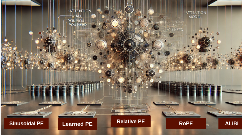
The exponential progress of models built in recent years is deeply connected with the advent of the Transformer architecture. Previously, AI scientists had to select architectures for each task at hand, and then optimize the hyper-parameters to get the best performance out of it. Another challenge limiting their potential was the difficulty in handling long-range dependencies of the data, surfacing the issues of vanishing gradients, loss of context over long sequences, and the inability to capture global context due to locality constraints. Additionally, the lack of scalability and parallelization in traditional models slowed training on large datasets, holding back the progress in the field.
The Transformer architecture revolutionized the field by addressing these issues through its self-attention mechanism. It enabled models to capture relationships over long sequences and efficiently understand global context, all while being highly parallelizable and adaptable across various modalities, such as text, images, and more. In the self-attention mechanism, for each token, its query is compared against the keys of all other tokens to compute similarity scores. These similarities are then used to weigh the value vectors, which ultimately decide where the current token should attend to. Self-attention treats all tokens as equally important regardless of their order, losing critical information about the sequence in which tokens appear, and in other words, it sees the input data as a set with no order. Now we need a mechanism to enforce some notion of order on the data, as natural language and many other types of data are inherently sequential and position-sensitive. This is where positional embeddings come into play. Positional embeddings encode the position of each token in the sequence, enabling the model to maintain awareness of the sequence’s structure. Various methods for encoding positional information have been explored, and we will cover them in this blog post.
Image generated by DALL-E
Attention Mechanism:
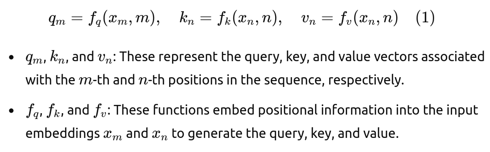
Let S = {wi} for i =1,…,N be a sequence of N input tokens where wi represents the i-th token. Hence, the corresponding token embedding of S can be denoted as E = {xi} for i =1,…,N where xi is the d-dimensional token embedding vector for token wi. The self-attention mechanism incorporates position embedding into token embeddings and generates the query, key, and value representations as:
Then, the attention weights is computed based on the similarity between query and key vectors:
The attention weights determine how important token n is for token m. In the other words, how much attention token m should pay to token n. The output for token m is computed as a weighted sum of the value vectors:
Therefore, the attention mechanism token m to gather information from other tokens in the sequence.
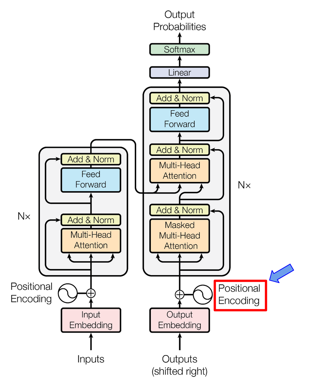
Fig 1. Positional encoding in transformer architecture (image from paper).
1. Absolute Position Embedding:
A typical choice for the equation (1) is to have:
Where pi is a d-dimensional vector, representing the absolute position of token xi. Sinusoidal positional encoding and learned positional encoding are two alternatives to generate pi.
1.a Sinusoidal Positional Encoding
Sinusoidal positional encoding was introduced in the “Attention is all you need” paper where transformer architecture was proposed. Sinusoidal Positional Encoding provides a unique position representation for each token in the input sequence. It is based on sine and cosine functions with different frequencies as:
Where pos is the position of the token in the sequence, d is the position embedding dimension, and i is the dimension index (0<=i<d).
The use of sine and cosine functions in sinusoidal positional encoding has a deep relationship with the Fourier transform. By using a range of different frequencies to encode positions, the Transformer creates a representation similar to a Fourier transform where:
High-frequency components (lower i) enable the model to capture local positional information. This is useful for understanding relationships between neighbor tokens in a sequence, such as word pairs.
Low-frequency components (higher i) capture more global patterns over the entire sequence. This helps the model to focus on broader relationships between tokens that may be far apart, such as dependencies between words in two different sentences.
This helps the model understand the relative positions of tokens by comparing their positional encodings. Sinusoidal positional encoding needs no additional training parameters while generalizing to larger sequence lengths at inference time. However, its expressiveness is limited.
1.b Learned Positional Encoding
Learned positional encoding was introduced in the “Attention is all you need” paper and it was applied in the BERT and GPT models as an alternative to Sinusoidal positional encoding. In learned positional encoding, each position in the sequence (e.g. first token, second token, etc) is assigned an embedding vector. These position embeddings are learned along with other transformer parameters during training. For example, if the model has a context length of 512 with a token embedding of size 768 (i.e. d=768), a learnable tensor of size 512*768 will be added to the other trainable parameters. This means the model gradually learns the best way to encode positional information for the specific task, such as text classification or translation.
Learned positional embedding is more expressive than sinusoidal one as the model can learn a position embedding, effective for its specific task. However, they introduce more trainable parameters which increases the model size and its computational cost.
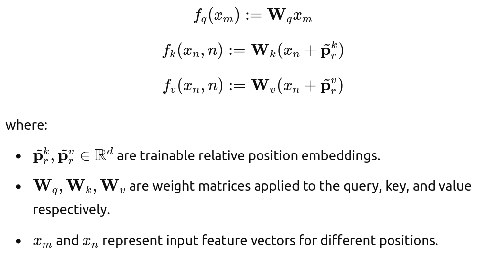
2. Relative Positional Embeddings
Both sinusoidal and learned position encodings focused on the absolute position of the token. However, the attention mechanism works by computing how important other tokens are for each specific token in the sequence. Hence, this process depends on the relative position of the tokens (how far apart they are from each other), rather than the absolute position of the tokens. To address the limitations of absolute position embedding, relative position encoding was introduced.
RelativePosEmb doesn’t add position information to token embeddings. Instead, it modifies the way key and value are computed at every layer as:
Here, r = clip(m-n, Rmin, Rmax) represents the relative distance between position m and n. The maximum relative position is clipped, assuming that precise relative position is not useful beyond a certain distance. Clipping the maximum distance enables the model to extrapolate at inference time, i.e. to generalize to sequence length not seen during training. However, this approach may miss some useful information from the absolute position of the token (like the position of the first token).
You may notice that fq lacks position embedding. That’s because we are encoding the relative position. In the attention formula, the query and key values are used to compute attention weights as equation (2) therefore we only need either the query or the key to include the relative position embedding.
This encoding has been used in many models as Transformer-XL and T5. There are different alternatives in applying relative positional encoding that you can find in papers [7] and [8] .
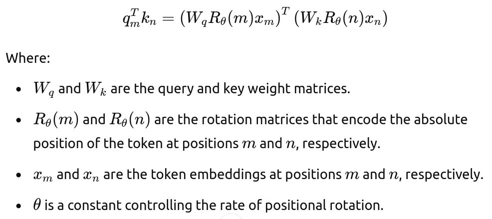
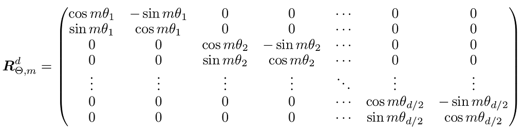
3. Rotary Positional Embedding (RoPE)
Unlike previous methods, RoPE rotates the vectors in a multi-dimensional space based on the position of tokens. Instead of adding position information to token embeddings, it modifies the way attention weights are computed at every layer as:
They proposed a generalized rotation matrix to any even embedding dimensionality d as:
Note that RoPE formulation doesn’t add position information to the values in the attention module. The output of the attention module is a weighted sum of the value vector and since position information isn’t added to values, the outputs of each transformer layer don’t have explicit position details.
Fig 2: ALiBi method visualization (image from paper).
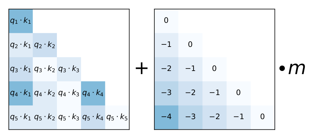
4. Attention with Linear Biases (ALiBi)
ALiBi also does not add positional encodings to word embeddings; instead, it adds a penalty to attention weight scores that is proportional to the distance between tokens. Therefore, the attention score between two tokens i and j at every layer is calculated as:
Attention score = query_i . key_j — m.(i-j)
Where -m.(i-j) is a penalty which is proportional to the distance between token i and j. The scalar m is a head-specific slope fixed before training and its values for different heads are chosen as a geometric sequence. For example, for 8 head, m might be:
This means, the first head has a relatively large m so it penalizes far apart tokens more and focuses on recent tokens, while the 8th head has the smallest m, allowing it to attend to more distant tokens. Fig. 2 also offers visualization.
Transformer extrapolation at inference time is the model’s ability to perform well to input sequences that are longer than those it was trained on. The transformer mechanism is agnostic to input length which means at inference time, it can work with longer sequences. However, note that the computational cost grows quadratically with input length even though the transformer layers themselves are agnostic to it.
The authors of ALiBi demonstrated that the bottleneck for transformer extrapolation is its position embedding method. As shown in Fig. 3, they compared the extrapolation capabilities of different position embedding methods. Since learned position embedding does not have a capability to encode positions greater than the training length, it has no extrapolation ability.
Fig 3: Extrapolation: as the input sequence gets longer (x-axis), sinusoidal, RoPE, and T5 position encodings show degraded perplexity (y-axis, lower is better), while ALiBi does not (image from paper).
Fig. 3 shows that the sinusoidal position embedding in practice has very limited extrapolation capabilities. While RoPE outperforms the sinusoidal one, it still does not achieve satisfactory results. The T5 bias method (a version of relative position embedding) leads to better extrapolation than both sinusoidal and RoPE embedding. Unfortunately, the T5 bias is computationally expensive (Fig. 4). ALiBi outperforms all these position embeddings with negligible (0–0.7%) memory increase.
Fig. 4: comparison of batched training, inference speed and memory use of sinusoidal, RoPE, T5, and ALiBi position encodings (image from paper).
Conclusion:
In summary, the way positional information is being encoded in Transformer architecture significantly affects its ability to understand sequential data, especially its extrapolation at inference time. While absolute positional embedding methods provide positional awareness, they often struggle with Transformer extrapolation. That’s why newer position embeddings are proposed. Relative position encoding, RoPE, and ALiBi have the capability to extrapolate at inference time. As transformers continue to be integrated in various applications, refining position encoding is crucial to push the boundaries of their performance.
The opinions expressed in this blog post are solely our own and do not reflect those of our employer.
References:
[1] Vaswani, A. “Attention is all you need.” (2017). [2] BERT: Devlin, Jacob. “Bert: Pre-training of deep bidirectional transformers for language understanding.” (2018). [3] GPT: Radford, Alec, et al. “Language models are unsupervised multitask learners.” (2019). [4] RelativePosEmb: Shaw, Peter, et al. “Self-attention with relative position representations.” (2018). [5] Transformer-XL Dai, Zihang. “Transformer-xl: Attentive language models beyond a fixed-length context.” (2019). [6] T5: Raffel, Colin, et al. “Exploring the limits of transfer learning with a unified text-to-text transformer.” (2020). [7] Raffel, Colin, et al. “Exploring the limits of transfer learning with a unified text-to-text transformer.” (2020) [8] He, Pengcheng, et al. “Deberta: Decoding-enhanced bert with disentangled attention.” (2020). [9] RoPE: Su, Jianlin, et al. “Roformer: Enhanced transformer with rotary position embedding.” (2024). [10] LLaMA: Touvron, Hugo, et al. “Llama: Open and efficient foundation language models.” (2023). [11] GPT-NeoX: Black, Sid, et al. “Gpt-neox-20b: An open-source autoregressive language model.” (2022). [12] ALiBi: Press, Ofir, et al. “Train short, test long: Attention with linear biases enables input length extrapolation.” (2021). [13] BloombergGPT: Wu, Shijie, et al. “Bloomberggpt: A large language model for finance.” (2023). [14] BLOOM: Le Scao, Teven, et al. “Bloom: A 176b-parameter open-access multilingual language model.” (2023).
Find closed-form solutions when possible — use numerical methods when necessary
A Python Refereeing an Italian Renaissance Mathematics Duel — Source: https://openai.com/dall-e-2/. All other figures from the author.
Why can we solve some equations easily, while others seem impossible? And another thing: why is this knowledge hidden from us?
As data scientists, applied scientists, and engineers, we often create mathematical models. For example, consider the model: y = x². Given a value for x, we can apply it forward to compute y. For instance, if x = 3, then y = 9.
We can also apply this model backward. Starting with y = x², we rearrange to solve for x: x = ±√y. If y = 9, then x = ±3. The expression x = ±√y is an example of a closed-form solution — an expression that uses a finite combination of standard operations and functions.
However, not all models are so straightforward. Sometimes, we encounter equations where we can’t simply “solve for x” and get a closed-form expression. In such cases, we might hear, “That’s not solvable — you need numerical methods.” Numerical methods are powerful. They can provide precise approximations. Still, it frustrates me (and perhaps you) that no one ever seems to explain when closed-form solutions are possible and when they aren’t.
The great Johannes Kepler shared our frustration. When studying planetary motion, he created this model:
y = x −c sin(x)
This equation converts a body’s position along its orbit (x) into its time along the orbit (y). Kepler sought a closed-form solution for x to turn time into a position. However, even 400 years later, the best we have are numerical methods.
In this article, we’ll build intuition about when to expect a closed-form solution. The only way to determine this rigorously is by using advanced mathematics — such as Galois theory, transcendental number theory, and algebraic geometry. These topics go far beyond what we, as applied scientists and engineers, typically learn in our training.
Instead of diving into these advanced fields, we’ll cheat. Using SymPy, a Python-based computer algebra system, we’ll explore different classes of equations to see which it can solve with a closed-form expression. For completeness, we’ll also apply numerical methods.
We’ll explore equations that combine polynomials, exponentials, logarithms, and trigonometric functions. Along the way, we’ll discover specific combinations that often resist closed-form solutions. We’ll see that if you want to create an equation with (or without) a closed-form solution, you should avoid (or try) the following:
Fifth degree and higher polynomials
Mixing x with exp(x) or log(x) — if Lambert’s W function is off-limits
Combining exp(x) and log(x) within the same equation
Some pairs of trigonometric functions with commensurate frequencies
Many pairs of trigonometric functions with non-commensurate frequencies
Mixing trigonometric functions with x, exp(x), or log(x)
Aside 1: I’m not a mathematician, and my SymPy scripts are not higher mathematics. If you find any mistakes or overlooked resources, forgive my oversight. Please share them with me, and I’ll gladly add a note.
Aside 2: Welch Lab’s recent video, Kepler’s Impossible Equation, reminded me of my frustration about not knowing when an equation can be solved in a closed form. The video sparked the investigation that follows and provides our first example.
Kepler’s Equation
Imagine you are Johannes Kepler’s research programmer. He has created the following model of orbital motion:
y = x −c sin(x)
where:
x is the body’s position along its orbit. We measure this position as an angle (in radians). The angle starts at 0 radians when the body is closest to the Sun. When the body has covered ¼ of its orbit’s distance, the angle is π/2 radians (90°). When it has covered half of its orbit’s distance, the angle is π (180°), and so on. Recall that radians measure angles from 0 to 2π rather than from 0 to 360°.
c is the orbit’s eccentricity, ranging from 0 (a perfect circle) to just under 1 (a highly elongated ellipse). Suppose Kepler has observed a comet with c = 0.967.
y is the body’s time along its orbit. We measure this time as an angle (in radians). For instance, if the comet has an orbital period of 76 Earth years, then π/2 (90°) corresponds to ¼ of 76 years, or 19 years. A time of π (180°) corresponds to ½ of 76 years, or 38 years. A time of 2π (360°) is the full 76-year orbital period.
This diagram shows the comet’s position at π/2 radians (90°), which is ¼ of the way along its orbit:
Kepler asks for the time when the comet reaches position π/2 radians (90°). You create and run this Python code:
t_earth_years = (time_radians / (2 * np.pi)) * orbital_period_earth_years print(f"It takes approximately {t_earth_years:.2f} Earth years for the comet to move from 0 to π/2 radians.")
You report back to Kepler:
It takes approximately 7.30 Earth years for the comet to move from 0 to π/2 radians.
Aside: The comet covers 25% of its orbit distance in under 10% of its orbital period because it speeds up when closer to the Sun.
No good deed goes unpunished. Kepler, fascinated by the result, assigns you a new task: “Can you tell me how far along its orbit the comet is after 20 Earth years? I want to know the position in radians.”
“No problem,” you think. “I’ll just use a bit of high school algebra.”
First, you convert 20 Earth years into radians:
time_radians = (20 / 76) × 2π = (10 / 19)π
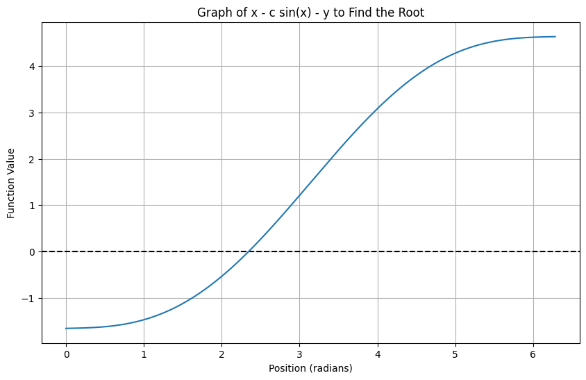
Next, you rearrange Kepler’s equation, setting it equal to 0.
x − 0.967 sin(x) − (10 / 19)π = 0
Now you want to find the value of x that makes this equation true. You decide to graph the equation to see where it crosses zero:
import numpy as np import matplotlib.pyplot as plt
def function_to_plot(x): return x - c * np.sin(x) - time_radians
x_vals = np.linspace(0, 2 * np.pi, 1000) function_values = function_to_plot(x_vals) plt.figure(figsize=(10, 6)) plt.axhline(0, color='black', linestyle='--') # dashed horizontal line at y=0 plt.xlabel("Position (radians)") plt.ylabel("Function Value") plt.title("Graph of x - c sin(x) - y to Find the Root") plt.grid(True)
plt.plot(x_vals, function_values) plt.show()
So far, so good. The graph shows that a solution for x exists. But when you try to rearrange the equation to solve for x using algebra, you hit a wall. How do you isolate x when you have a combination of x and sin(x)?
“That’s okay,” you think. “We’ve got Python, and Python has the SymPy package,” a powerful and free computer algebra system.
You pose the problem to SymPy:
# Warning: This code will fail. import sympy as sym from sympy import pi, sin from sympy.abc import x
c = 0.967 time_earth_years = 20 orbital_period_earth_years = 76
time_radians = (time_earth_years / orbital_period_earth_years) * 2 * pi equation = x - c * sin(x) - time_radians
NotImplementedError: multiple generators [x, sin(x)]
No algorithms are implemented to solve equation x - 967*sin(x)/1000 - 10*pi/19
SymPy is quite good at solving equations, but not all equations can be solved in what’s called closed form — a solution expressed in a finite number of elementary functions such as addition, multiplication, roots, exponentials, logarithms, and trigonometric functions. When we combine a term such as x with a trigonometric term like sin(x), isolating x can become fundamentally impossible. In other words, these types of mixed equations often lack a closed-form solution.
That’s okay. From the graph, we know a solution exists. SymPy can get us arbitrarily close to that solution using numerical methods. We use SymPy’s nsolve():
import sympy as sym
from sympy import pi, sin
from sympy.abc import x

c = 0.967
time_earth_years = 20
orbital_period_earth_years = 76
time_radians = (time_earth_years / orbital_period_earth_years) * 2 * pi
equation = x - c * sin(x) - time_radians

initial_guess = 1.0   # Initial guess for the numerical solver
position_radians = sym.nsolve(equation, x, initial_guess)
print(f"After {time_earth_years} Earth years, the comet will travel {position_radians:.4f} radians ({position_radians * 180 / pi:.2f}°) along its orbit.")
Which reports:
After 20 Earth years, the comet will travel 2.3449 radians (134.35°) along its orbit.
We can summarize the results in a table:
Are we sure there is not a closed-form solution? We add a question mark to our “No” answer. This reminds us that SymPy’s failure is not a mathematical proof that no closed-form solution exists. We label the last column “A Numeric” to remind ourselves that it represents one numerical solution. There could be more.
In this section, we explored Kepler’s equation and discovered the challenge of solving it in closed form. Python’s SymPy package confirmed our struggle, and in the end, we had to rely on a numerical solution.
This gives us one example of an equation with no apparent closed-form solution. But is this typical? Are there classes of equations where we can always — or never — find a closed-form solution? Let’s dig deeper by exploring another kind of equation: polynomials.
Polynomials
Polynomial equations such as x² − x − 1 = 0 are the reliable hammer of mathematical modeling — straightforward but powerful. We all learn how to solve degree-two polynomials (those with x², “quadratic”) in school.
500 years ago, during the Renaissance in Italy, solving polynomials of higher degrees became a form of public entertainment. Mathematicians like Tartaglia and Cardano competed for glory and recognition in public math duels. These contests led to solutions for degree-three (cubic) and degree-four (quartic) polynomials. But what about degree five?
Let’s use SymPy to investigate a sample of polynomials:
For polynomials up to degree four, we can always find closed-form elementary solutions. Specifically, these solutions require only a finite expression of basic arithmetic operations and roots (such as square roots or cube roots).
The number of solutions will never exceed the degree of the polynomial. However, some solutions may involve i, the square root of −1, which represents complex numbers. More on that in a moment.
And what about degree-five polynomials and beyond? Can we always find closed-form solutions? The answer is mixed. Sometimes, we can. When a closed-form solution exists — for example, for x⁵+1=0 above — SymPy typically finds it.
However, in other cases, such as with x⁵-x-1=0, SymPy cannot find a closed-form, elementary solution. Évariste Galois famously demonstrated the impossibility of closed-form solutions for general higher-degree polynomial. However, SymPy’s failure on a specific equation is not a proof that no closed-form solution exists. So, for this example, we add a question mark and answer “No?”.
To explore further, let’s see exactly what SymPy does when given x⁵-x-1=0:
[CRootOf(x**5 - x - 1, 0), CRootOf(x**5 - x - 1, 1), CRootOf(x**5 - x - 1, 2), CRootOf(x**5 - x - 1, 3), CRootOf(x**5 - x - 1, 4)]
Yikes! SymPy is clearly cheating here. It’s saying, “Oh, you want a closed form? No problem! I’ll just define a new, one-off function called CRootOf(x**5 – x – 1, 0) and call that the answer.”
This is cheating because it doesn’t answer the question of interest. SymPy is essentially giving a new name to an unsolved problem and claiming success.
SymPy, of course, has good reasons for producing its answer this way. For one thing, we can now easily find a numerical solution:
from sympy import N, CRootOf

print(N(CRootOf(x**5 - x - 1, 0)))
Prints 1.16730397826142.
Solutions Even When No Real Solutions Exist: One surprising thing about polynomial equations is that you can always find solutions — at least numerically — even when no real solutions exist!
Consider this simple equation of degree two:
x² + 1 = 0
If we plot this equation, it never crosses the x-axis, indicating no real solutions.
However, using SymPy, we can find numerical solutions for any polynomial. For example:
from sympy import solve, Eq, CRootOf, N, degree
from sympy.abc import x

equation = Eq(x**2 + 1, 0)
numerical_solution = [N(CRootOf(equation, d)) for d in range(degree(equation))]
print(numerical_solution)
Which prints: [-1.0*I, 1.0*I].
Notice that the solutions use i (the imaginary unit), meaning they are complex numbers. This is an illustration of the Fundamental Theorem of Algebra, which states that every (non-constant) polynomial equation has at least one complex solution, even when no real solutions exist.
The takeaway: unless complex numbers are meaningful in your domain, you should ignore complex solutions.
To summarize polynomials:
Degree four and below: There is always a closed-form solution involving basic arithmetic operations and roots.
Degree five and above: Generally, no closed-form solution exists using elementary operations, though SymPy occasionally finds one.
Solutions: Polynomials will always have solutions — at least numerically — but these solutions may not be real (both mathematically and practically). You should typically ignore them unless complex numbers are meaningful in your domain.
Next, we’ll add exponentials and logarithms to our equations. In the solutions, we discover the Lambert W function. Is it a CRootOf-like cheat?
Exp, Log and x
When we model data mathematically, we often use exponentials and logarithms. Below is a sample of what happens when we try to reverse such models by solving their equations with SymPy:
Observations:
Sometimes you get lucky: The first equation xeˣ=0 has an elementary solution x=0. While this isn’t always the case, simple closed-form solutions can sometimes be found, even in equations involving exponentials or logarithms.
Every equation in this “family” appears to be solvable, with two caveats: First, I can’t precisely define this family and am unsure if a clear definition is possible. Second, solving these equations requires the Lambert W function, such as W(1) and W₋₁(1/10). This function arises when x appears both inside and outside of an exponential (or logarithmic) expression.
If you don’t accept W, you can’t solve these functions in closed form: Equations in this “family” generally have no closed-form elementary solutions without the Lambert W function.
We should accept W: The Lambert W function is a well-defined, easily computable function with applications across math and science. Its late adoption relative to exp, log, sin, and cos is simply historical.
A single W can generate multiple solutions: Similar to how the square root function can produce two solutions, a W expression can yield zero, one, or two real solutions. When two real solutions exist, SymPy lists them separately, representing one as W (the principal branch) and the other as W₋₁ (the secondary branch). Beyond the real solutions, any W expression also generates an infinite number of complex solutions.
Complex solutions will arise: Some equations, such as x log(x)+1=0, lead to only complex solutions. As with polynomials, you should ignore complex numbers unless they are meaningful in your domain.
Degree-five and higher polynomials mixed with exp (or log) remain unsolvable: Even with special functions like the Lambert W function, degree-five and higher polynomials cannot be solved in closed form using elementary functions.
What happens if we use both an exponential and a logarithm in the same equation? Generally, we won’t find a closed-form solution — not even with the Lambert W function:
To summarize, combining exponentials or logarithms with polynomials typically makes the equation unsolvable by traditional closed-form methods. However, if we allow the Lambert W function, equations with exponentials or logarithms (but not both) become solvable. We should embrace W as a valid tool for handling such cases.
Next, let’s generalize Kepler’s problem and see what happens when we introduce trigonometric functions into our equations.
Trigonometric Equations
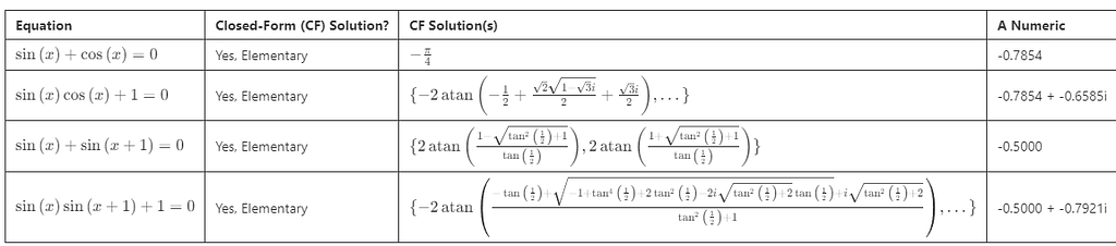
Simple Trigonometric Equations: Here is our first batch of trigonometric samples:
SymPy successfully finds closed-form elementary solutions for each equation. The solutions involve trigonometric functions, and in some cases, complex numbers appear. (Again, we typically ignore the complex solutions unless they are meaningful for the problem at hand.)
Keep in mind that sine and cosine are periodic, which leads to infinitely many solutions. The closed-form solutions that SymPy provides typically represent a single cycle.
Commensurate Frequency Equations: In the preceding equations, we limited the trigonometric function’s input to x+b, where b is a constant. What happens if we allow inputs like a₁x+b₁ and a₂x+b₂ where a₁ is rational and a₂ is rational? This means the two periodic functions may have different frequencies but those frequences can synchronize. (The a’s are the frequencies.) We say our trigonometric functions have “commensurate frequencies.”
Observations:
We occasionally get a closed-form elementary solution.
On sin(x) + sin(3x)+1=0, SymPy returns zero solutions. Plots and numerical methods, however, suggest solutions exist. Moreover, when I input sin(x) + sin(3x)+1=0 into WolframAlpha, an on-line computer algebra system, it produces hybrid solutions. (The WolframAlpha solutions combine elementary functions with CRootOf expressions of degree six. As we discussed in the polynomial section, such expressions generally lack a closed-form solution.)
SymPy sometimes times out looking for a closed-form solution when numerical methods can still provide solutions.
In other cases, it times out, and both numerical methods and plots confirm there are no solutions. Before, instead of no numerical solution, we’d get a complex number solution. [WolframAlpha does give a complex numerical solution.]
Let’s plot the equation that returned zero closed-formed solutions. Let’s also plot the one that numerically returned ValueError:
Additional Observations:
From the blue plot, SymPy’s response of “no solutions” appears to be a bug. There are clearly solutions in the plot, and SymPy should either have found them or thrown an exception.
On the other hand, in the red plot, the numerical result of ValueError is accurate. There are no solutions.
For all the trigonometric equations we’ve encountered so far, SymPy seems to find real-valued closed-form solutions when they exist. When they don’t exist, it times out or gives unpredictable errors.
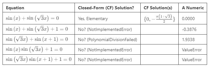
Non-Commensurate Frequency Equations: In the preceding equations, we allowed trigonometric functions with inputs of the form ax+b, where a is a rational constant. What happens if we allow inputs like a₁x+b₁ and a₂x+b₂ where a₁ is rational and a₂ is irrational? This means the two periodic functions will never synchronize. We say they have “non-commensurate frequencies.”
Observations:
Equations with two trigonometric functions having non-commensurate frequencies generally seem unsolvable in closed form. When no elementary solution is available, SymPy returns NotImplementedError.
We can still get lucky and occasionally find an equation with an elementary solution. In the case above, in which SymPy returned PolynomialDivisionFailed, WolframAlpha found a closed-form solution.
When an equation has no solutions, SymPy produces a ValueError, which we can confirm through plots (see below). We did not see complex-number results in these cases.
The equations do not quite touch zero, so no solutions
Our conclusion regarding trigonometric equations is that we can often find elementary closed-form solutions. The main exception seems to be when the frequencies are non-commensurate — for example, in an equation containing sin(x) and sin(√3 x).
The final question we’ll explore is what happens when we mix trigonometric functions with exponentials and logarithms.
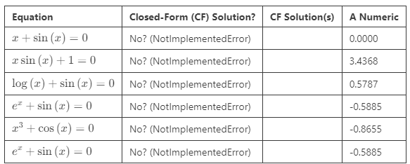
Trigonometric and x, Exp, Log
Our final set of samples will require only a short discussion. What if we run a sample of equations through SymPy, each equation containing one trigonometric function combined with either x, exp(x), or log(x)?
The results are unanimous: SymPy is unable to produce closed-form solutions for any of these combinations. However, it seems that SymPy should have produced x=0 as the closed-form solution for the first equation, as indeed WolframAlpha does.
Conclusion
So, there you have it — an exploration of which equations tend to lack closed-form solutions. If you’re interested in experimenting with the examples in this article, you can find my Python code on GitHub.
As I worked through these sample equations, here is what surprised me:
Kepler’s Equation is wonderfully simple. I didn’t know one could model anellipse — a geometric shape I find complicated — with such elegance.
Lambert’s W function proved to be invaluable for handling equations that mix terms like x and exp(x). We should consider it an elementary function.
SymPy is an excellent, free tool that handles symbolic algebra and trigonometric equations far better than many of us could handle manually. While it may not match WolframAlpha in some cases, it’s incredibly versatile and accessible.
Mixing trigonometric functions with other terms frequently prevents closed-form solutions, especially when frequencies are non-commensurate.
When closed-form solutions remain out of reach, plotting and numerical methods step in, delivering practical results.
Thank you for joining me on this journey. I hope you now have a clearer understanding of when you can use equation-solving techniques to reverse models and how much SymPy can assist. Also, when an equation resists a closed-form solution, you can now understand why and when to rely on numerical methods.
If you enjoyed exploring mathematics with Python and SymPy, you may also enjoy using them to explore Newtonian physics. Please see thisTowards Data Science article and the related, popular PyData conference talk.
Interested in future articles? Please follow me on Medium. I write about Rust and Python, scientific programming, machine learning, and statistics. I tend to write about one article per month.
We use cookies on our website to give you the most relevant experience by remembering your preferences and repeat visits. By clicking “Accept”, you consent to the use of ALL the cookies.
This website uses cookies to improve your experience while you navigate through the website. Out of these, the cookies that are categorized as necessary are stored on your browser as they are essential for the working of basic functionalities of the website. We also use third-party cookies that help us analyze and understand how you use this website. These cookies will be stored in your browser only with your consent. You also have the option to opt-out of these cookies. But opting out of some of these cookies may affect your browsing experience.
Necessary cookies are absolutely essential for the website to function properly. These cookies ensure basic functionalities and security features of the website, anonymously.
Cookie
Duration
Description
cookielawinfo-checkbox-analytics
11 months
This cookie is set by GDPR Cookie Consent plugin. The cookie is used to store the user consent for the cookies in the category "Analytics".
cookielawinfo-checkbox-functional
11 months
The cookie is set by GDPR cookie consent to record the user consent for the cookies in the category "Functional".
cookielawinfo-checkbox-necessary
11 months
This cookie is set by GDPR Cookie Consent plugin. The cookies is used to store the user consent for the cookies in the category "Necessary".
cookielawinfo-checkbox-others
11 months
This cookie is set by GDPR Cookie Consent plugin. The cookie is used to store the user consent for the cookies in the category "Other.
cookielawinfo-checkbox-performance
11 months
This cookie is set by GDPR Cookie Consent plugin. The cookie is used to store the user consent for the cookies in the category "Performance".
viewed_cookie_policy
11 months
The cookie is set by the GDPR Cookie Consent plugin and is used to store whether or not user has consented to the use of cookies. It does not store any personal data.
Functional cookies help to perform certain functionalities like sharing the content of the website on social media platforms, collect feedbacks, and other third-party features.
Performance cookies are used to understand and analyze the key performance indexes of the website which helps in delivering a better user experience for the visitors.
Analytical cookies are used to understand how visitors interact with the website. These cookies help provide information on metrics the number of visitors, bounce rate, traffic source, etc.
Advertisement cookies are used to provide visitors with relevant ads and marketing campaigns. These cookies track visitors across websites and collect information to provide customized ads.