Blog

Is it better than grid search?

When I notice my model is overfitting, I often think, “It is time to regularize”. But how do I decide which regularization method to use (L1, L2) and what parameters to choose? Typically, I perform hyperparameter optimization by means of a grid search to select the settings. However, what happens if the independent variables have different scales or varying levels of influence? Can I design a hyperparameter grid with different regularization coefficients for each variable? Is this type of optimization feasible in high-dimensional spaces? And are there alternative ways to design regularization? Let’s explore this with a hypothetical example.

Use case

My fictional example is a binary classification use case with 3 explanatory variables. Each of these variables is categorical and has 7 different categories. My reproducible use case is in this notebook. The function that generates the dataset is the following:

import numpy as np
import pandas as pd

def get_classification_dataset():
    n_samples = 200
    cats = ["a", "b", "c", "d", "e", "f"]
    X = pd.DataFrame(
        data={
            "col1": np.random.choice(cats, size=n_samples),
            "col2": np.random.choice(cats, size=n_samples),
            "col3": np.random.choice(cats, size=n_samples),
        }
    )
    X_preprocessed = pd.get_dummies(X)

    theta = np.random.multivariate_normal(
        np.zeros(len(cats) * X.shape[1]),
        np.diag(np.array([1e-1] * len(cats) + [1] * len(cats) + [1e1] * len(cats))),
    )

    y = pd.Series(
        data=np.random.binomial(1, expit(np.dot(X_preprocessed.to_numpy(), theta))),
        index=X_preprocessed.index,
    )
    return X_preprocessed, y

For information, I deliberately chose 3 different values for the theta covariance matrix to showcase the benefit of the Laplace approximated bayesian optimization method. If the values were somehow similar, the interest would be minor.

Benchmark

Along with a simple baseline model that predicts the mean observed value on the training dataset (used for comparison purposes), I opted to design a slightly more complex model. I decided to one-hot encode the three independent variables and apply a logistic regression model on top of this basic preprocessing. For regularization, I chose an L2 design and aimed to find the optimal regularization coefficient using two techniques: grid search and Laplace approximated bayesian optimization, as you may have anticipated by now. Finally, I evaluated the model on a test dataset using two metrics (arbitrarily selected): log loss and AUC ROC.

Before presenting the results, let’s first take a closer look at the bayesian model and how we optimize it.

Bayesian model

In the bayesian framework, the parameters are no longer fixed constants, but random variables. Instead of maximizing the likelihood to estimate these unknown parameters, we now optimize the posterior distribution of the random parameters, given the observed data. This requires us to choose, often somewhat arbitrarily, the design and parameters of the prior. However, it is also possible to treat the parameters of the prior as random variables themselves — like in Inception, where the layers of uncertainty keep stacking on top of each other…

In this study, I have chosen the following model:

I have logically chosen a bernouilli model for Y_i | θ, a normal centered prior corresponding to a L2 regularization for θ | Σ and finally for Σ_i^{-1}, I chose a Gamma model. I chose to model the precision matrix instead of the covariance matrix as it is traditional in the literature, like in scikit learn user guide for the Bayesian linear regression [2].

In addition to this written model, I assumed the Y_i and Y_j are conditionally (on θ) independent as well as Y_i and Σ.

Calibration

Likelihood

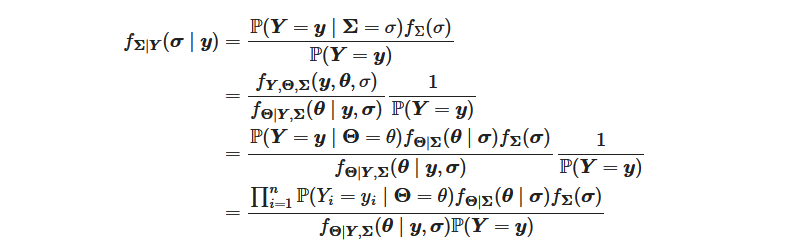
According to the model, the likelihood can consequently be written:

In order to optimize, we need to evaluate nearly all of the terms, with the exception of P(Y=y). The terms in the numerators can be evaluated using the chosen model. However, the remaining term in the denominator cannot. This is where the Laplace approximation comes into play.

Laplace approximation

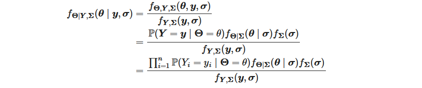
In order to evaluate the first term of the denominator, we can leverage the Laplace approximation. We approximate the distribution of θ | Y, Σ by:

with θ* being the mode of the mode the density distribution of θ | Y, Σ.

Even though we do not know the density function, we can evaluate the Hessian part thanks to the following decomposition:

We only need to know the first two terms of the numerator to evaluate the Hessian which we do.

For those interested in further explanation, I advise part 4.4, “The Laplace Approximation”, from Pattern Recognition and Machine Learning from Christopher M. Bishop [1]. It helped me a lot to understand the approximation.

Laplace approximated likelihood

Finally the Laplace approximated likelihood to optimize is:

Once we approximate the density function of θ | Y, Σ, we could finally evaluate the likelihood at whatever θ we want if the approximation was accurate everywhere. For the sake of simplicity and because the approximation is accurate only close to the mode, we evaluate approximated likelihood at θ*.

Here after is a function that evaluates this loss for a given (scalar) σ²=1/p (in addition to the given observed, X and y, and design values, α and β).

import numpy as np
from scipy.stats import gamma

from module.bayesian_model import BayesianLogisticRegression

def loss(p, X, y, alpha, beta):
    # computation of the loss for given values:
    # - 1/sigma² (named p for precision here)
    # - X: matrix of features
    # - y: vector of observations
    # - alpha: prior Gamma distribution alpha parameter over 1/sigma²
    # - beta: prior Gamma distribution beta parameter over 1/sigma²

    n_feat = X.shape[1]
    m_vec = np.array([0] * n_feat)
    p_vec = np.array(p * n_feat)

    # computation of theta*
    res = minimize(
        BayesianLogisticRegression()._loss,
        np.array([0] * n_feat),
        args=(X, y, m_vec, p_vec),
        method="BFGS",
        jac=BayesianLogisticRegression()._jac,
    )
    theta_star = res.x
    
    # computation the Hessian for the Laplace approximation
    H = BayesianLogisticRegression()._hess(theta_star, X, y, m_vec, p_vec)
    
    # loss
    loss = 0
    ## first two terms: the log loss and the regularization term
    loss += baysian_model._loss(theta_star, X, y, m_vec, p_vec)
    ## third term: prior distribution over sigma, written p here
    out -= gamma.logpdf(p, a = alpha, scale = 1 / beta)
    ## fourth term: Laplace approximated last term
    out += 0.5 * np.linalg.slogdet(H)[1] - 0.5 * n_feat * np.log(2 * np.pi)

    return out

In my use case, I have chosen to optimize it by means of Adam optimizer, which code has been taken from this repo.

def adam(
    fun,
    x0,
    jac,
    args=(),
    learning_rate=0.001,
    beta1=0.9,
    beta2=0.999,
    eps=1e-8,
    startiter=0,
    maxiter=1000,
    callback=None,
    **kwargs
):
    """``scipy.optimize.minimize`` compatible implementation of ADAM -
    [http://arxiv.org/pdf/1412.6980.pdf].
    Adapted from ``autograd/misc/optimizers.py``.
    """
    x = x0
    m = np.zeros_like(x)
    v = np.zeros_like(x)

    for i in range(startiter, startiter + maxiter):
        g = jac(x, *args)

        if callback and callback(x):
            break

        m = (1 - beta1) * g + beta1 * m  # first  moment estimate.
        v = (1 - beta2) * (g**2) + beta2 * v  # second moment estimate.
        mhat = m / (1 - beta1**(i + 1))  # bias correction.
        vhat = v / (1 - beta2**(i + 1))
        x = x - learning_rate * mhat / (np.sqrt(vhat) + eps)

    i += 1
    return OptimizeResult(x=x, fun=fun(x, *args), jac=g, nit=i, nfev=i, success=True)

For this optimization we need the derivative of the previous loss. We cannot have an analytical form so I decided to use a numerical approximation of the derivative.

Inference

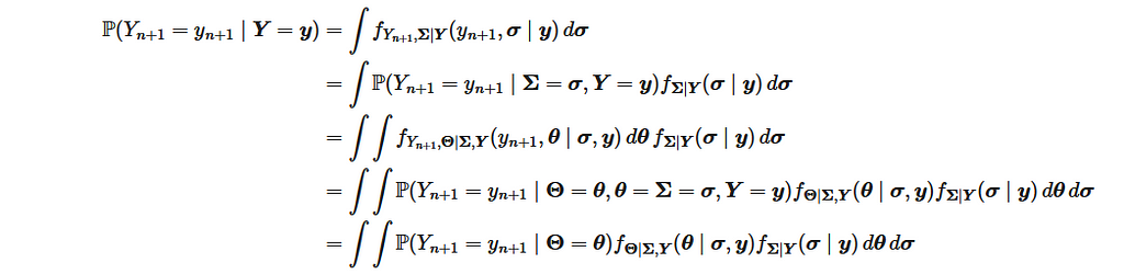
Once the model is trained on the training dataset, it is necessary to make predictions on the evaluation dataset to assess its performance and compare different models. However, it is not possible to directly calculate the actual distribution of a new point, as the computation is intractable.

It is possible to approximate the results with:

considering:

Results

I chose an uninformative prior over the precision random variable. The naive model performs poorly, with a log loss of 0.60 and an AUC ROC of 0.50. The second model performs better, with a log loss of 0.44 and an AUC ROC of 0.83, both when hyperoptimized using grid search and bayesian optimization. This indicates that the logistic regression model, which incorporates the dependent variables, outperforms the naive model. However, there is no advantage to using bayesian optimization over grid search, so I’ll continue with grid search for now. Thanks for reading.

… But wait, I am thinking. Why are my parameters regularized with the same coefficient? Shouldn’t my prior depend on the underlying dependent variables? Perhaps the parameters for the first dependent variable could take higher values, while those for the second dependent variable, with its smaller influence, should be closer to zero. Let’s explore these new dimensions.

Benchmark 2

So far we have considered two techniques, the grid search and the bayesian optimization. We can use these same techniques in higher dimensions.

Considering new dimensions could dramatically increase the number of nodes of my grid. This is why the bayesian optimization makes sense in higher dimensions to get the best regularization coefficients. In the considered use case, I have supposed there are 3 regularization parameters, one for each independent variable. After encoding a single variable, I assumed the generated new variables all shared the same regularization parameter. Hence the total regularization parameters of 3, even if there are more than 3 columns as inputs of the logistic regression.

I updated the previous loss function with the following code:

import numpy as np
from scipy.stats import gamma

from module.bayesian_model import BayesianLogisticRegression

def loss(p, X, y, alpha, beta, X_columns, col_to_p_id):
    # computation of the loss for given values:
    # - 1/sigma² vector (named p for precision here)
    # - X: matrix of features
    # - y: vector of observations
    # - alpha: prior Gamma distribution alpha parameter over 1/sigma²
    # - beta: prior Gamma distribution beta parameter over 1/sigma²
    # - X_columns: list of names of X columns
    # - col_to_p_id: dictionnary mapping a column name to a p index
    # because many column names can share the same p value

    n_feat = X.shape[1]
    m_vec = np.array([0] * n_feat)
    p_list = []
    for col in X_columns:
        p_list.append(p[col_to_p_id[col]])
    p_vec = np.array(p_list)

    # computation of theta*
    res = minimize(
        BayesianLogisticRegression()._loss,
        np.array([0] * n_feat),
        args=(X, y, m_vec, p_vec),
        method="BFGS",
        jac=BayesianLogisticRegression()._jac,
    )
    theta_star = res.x
    
    # computation the Hessian for the Laplace approximation
    H = BayesianLogisticRegression()._hess(theta_star, X, y, m_vec, p_vec)
    
    # loss
    loss = 0
    ## first two terms: the log loss and the regularization term
    loss += baysian_model._loss(theta_star, X, y, m_vec, p_vec)
    ## third term: prior distribution over 1/sigma² written p here
    ## there is now a sum as p is now a vector
    out -= np.sum(gamma.logpdf(p, a = alpha, scale = 1 / beta))
    ## fourth term: Laplace approximated last term
    out += 0.5 * np.linalg.slogdet(H)[1] - 0.5 * n_feat * np.log(2 * np.pi)

    return out

With this approach, the metrics evaluated on the test dataset are the following: 0.39 and 0.88, which are better than the initial model optimized by means of a grid search and a bayesian approach with only a single prior for all the independent variables.

The use case can be reproduced with this notebook.

Limits

I have created an example to illustrate the usefulness of the technique. However, I have not been able to find a suitable real-world dataset to fully demonstrate its potential. While I was working with an actual dataset, I could not derive any significant benefits from applying this technique. If you come across one, please let me know — I would be excited to see a real-world application of this regularization method.

Conclusion

In conclusion, using bayesian optimization (with Laplace approximation if needed) to determine the best regularization parameters may be a good alternative to traditional hyperparameter tuning methods. By leveraging probabilistic models, bayesian optimization not only reduces the computational cost but also enhances the likelihood of finding optimal regularization values, especially in high dimension.

References

1. Christopher M. Bishop. (2006). Pattern Recognition and Machine Learning. Springer.
2. Bayesian Ridge Regression scikit-learn user guide: https://scikit-learn.org/1.5/modules/linear_model.html#bayesian-ridge-regression

Exploring New Hyperparameter Dimensions with Laplace Approximated Bayesian Optimization was originally published in Towards Data Science on Medium, where people are continuing the conversation by highlighting and responding to this story.