MapleStory Universe enters its eagerly awaited second Pioneer Test to optimize system stability and gather stakeholders’ feedback before the official launch. According to the announcement made earlier today by NEXPACA, an innovative blockchain company, the Open Beta Test will start on November 202nd, 2024, and end on November 29th, 2024. Notably, MapleStory Universe has created […]
Slovenia’s historic city of Maribor is the location for this week’s NiceHashX, a Bitcoin-focused conference organized by the eponymous hashrate marketplace. The two-day event, dubbed ‘the Bitcoin Conference on the Sunny Side of the Alps,’ comes at a pivotal moment for the world’s leading digital currency, which recently came within a whisker of surpassing its […]
Relighting is the task of rendering a scene under a specified target lighting condition, given an input scene. This is a crucial task in computer vision and graphics. However, it is an ill-posed problem, because the appearance of an object in a scene results from a complex interplay between factors like the light source, the geometry, and the material properties of the surface. These interactions create ambiguities. For instance, given a photograph of a scene, is a dark spot on an object due to a shadow cast by lighting or is the material itself dark in color? Distinguishing between these factors is key to effective relighting.
In this blog post we discuss how different papers are tackling the problem of relighting via diffusion models. Relighting encompases a variety of subproblems including simple lighting adjustments, image harmonization, shadow removal and intrinsic decomposition. These areas are essential for refining scene edits such as balancing color and shadow across composited images or decoupling material and lighting properties. We will first introduce the problem of relighting and briefly discuss Diffusion models and ControlNets. We will then discuss different approaches that solve the problem of relighting in different types of scenes ranging from single objects to portraits to large scenes.
Solving Relighting
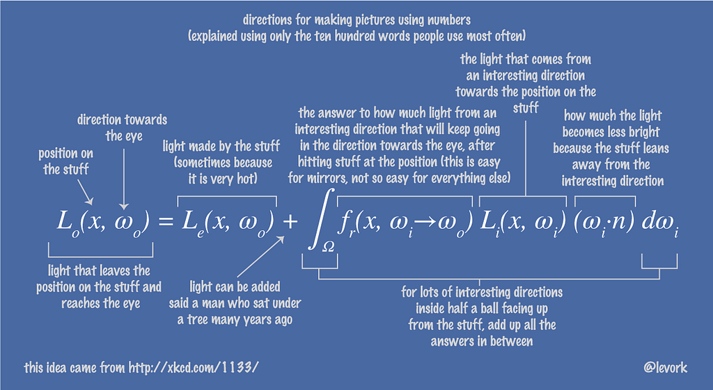
The goal is to decompose the scene into its fundamental components such as geometry, material, and light interactions and model them parametrically. Once solved then we can change it according to our preference. The appearance of a point in the scene can be described by the rendering equation as follows:
Most methods aim to solve for each single component of the rendering equation. Once solved, then we can perform relighting and material editing. Since the lighting term L is on both sides, this equation cannot be evaluated analytically and is either solved via Monte Carlo methods or approximation based approaches.
An alternate approach is data-driven learning, where instead of explicitly modeling the scene properties it directly learns from data. For example, instead of fitting a parametric function, a network can learn the material properties of the surface from data. Data-driven approaches have proven to be more powerful than parametric approaches. However they require a huge amount of high quality data which is really hard to collect especially for lighting and material estimation tasks.
Datasets for lighting and material estimation are rare as they require expensive, complex setups such as light stages to capture detailed lighting interactions. These setups are accessible to only a few organizations, limiting the availability of data for training and evaluation. There are no full-body ground truth light stage datasets publicly available which further highlights this challenge.
Diffusion Models
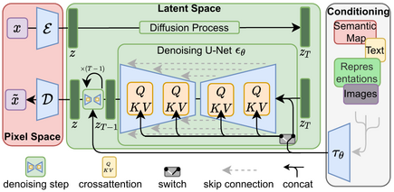
Computer vision has experienced a significant transformation with the advent of pre-training on vast amounts of image and video data available online. This has led to the development of foundation models, which serve as powerful general-purpose models that can be fine-tuned for a wide range of specific tasks. Diffusion models work by learning to model the underlying data distribution from independent samples, gradually reversing a noise-adding process to generate realistic data. By leveraging their ability to generate high-quality samples from learned distributions, diffusion models have become essential tools for solving a diverse set of generative tasks.
One of the most prominent examples of this is Stable Diffusion(SD), which was trained on the large-scale LAION-5B dataset that consists of 5 billion image text pairs. It has encoded a wealth of general knowledge about visual concepts making it suitable for fine-tuning for specific tasks. It has learnt fundamental relationships and associations during training such as chairs having 4 legs or recognizing structure of cars. This intrinsic understanding has allowed Stable Diffusion to generate highly coherent and realistic images and be used for fine tuning to predict other modalities. Based on this idea, the question arises if we can leverage pretrained SD to solve the problem of scene relighting.
So how do we fine-tune LDMs? A naive approach is to do transfer learning with LDMs. This would be freezing early layers (which capture general features) and fine tuning the model on the specific task. While this approach has been used by some papers such as Alchemist (for Material Transfer), it requires a large amount of paired data for the model to generalize well. Another drawback to this approach is the risk of catastrophic forgetting, where the model losses the knowledge gained during pretraining. This would limit its capability on generalizing across various conditions.
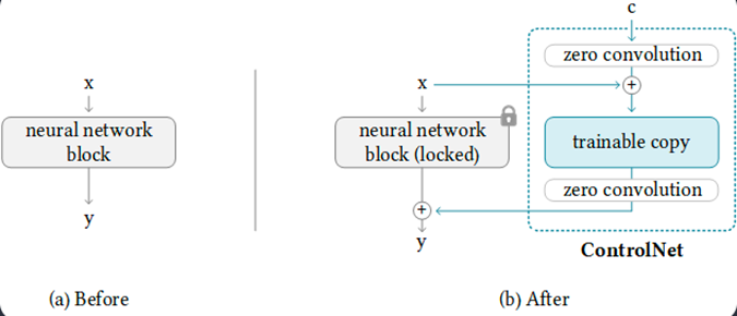
Another approach to fine-tuning such large models is by introducing a ControlNet. Here, a copy of the network is made and the weights of the original network are frozen. During training only the duplicate network weights are updated and the conditioning signal is passed as input to the duplicate network. The original network continues to leverage its pretrained knowledge.
While this increases the memory footprint, the advantage is that we dont lose the generalization capabilities acquired from training on large scale datasets. It ensures that it retains its ability to generate high-quality outputs across a wide range of prompts while learning the task specific relationships needed for the current task.
Additionally it helps the model learn robust and meaningful connections between control input and the desired output. By decoupling the control network from the core model, it avoids the risk of overfitting or catastrophic forgetting. It also needs significantly less paired data to train.
While there are other techniques for fine-tuning foundational models — such as LoRA (Low-Rank Adaptation) and others — we will focus on the two methods discussed: traditional transfer learning and ControlNet. These approaches are particularly relevant for understanding how various papers have tackled image-based relighting using diffusion models.
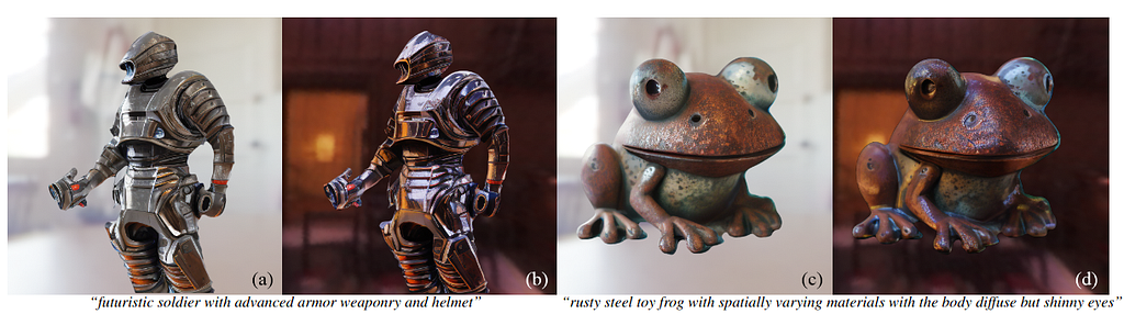
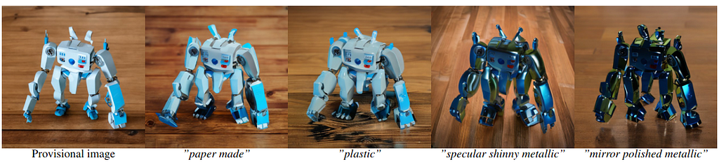
This work proposes fine grained control over relighting of an input image. The input image can either be generated or given as input. Further it can also change the material of the object based on the text prompt. The objective is to exert fine-grained control on the effects of lighting.
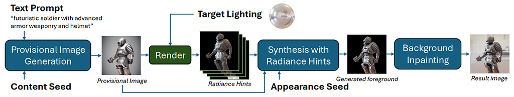
Given an input image, the following preprocessing steps are applied:
Estimate background and depth map using off the shelf SOTA models.
Extract mesh by triangulating the depth map
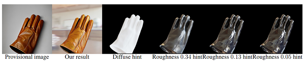
Generate 4 different radiance cues images. Radiance cues images are created by assigning the extracted mesh different materials and rendering them under target lighting. The radiance cues images act as basis for encoding lighting effects such as specular, shadows and global illumination.
Once these images are generated, they train a ControlNet module. The input image and the mask are passed through an encoder decoder network which outputs a 12 channel feature map. This is then multiplied with the radiance cues images that are channel wise concatenated together. Thus during training, the noisy target image is denoised with this custom 12 channel image as conditioning signal.
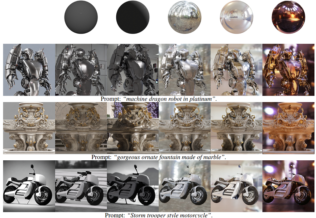
Additionally an appearance seed is provided to procure consistent appearance under different illumination. Without it the network renders a different interpretation of light-matter interaction. Additionally one can provide more cues via text to alter the appearance such as by adding “plastic/shiny metallic” to change the material of the generated image.
Implementation
The dataset was curated using 25K synthetic objects from Objaverse. Each object was rendered from 4 unique views and lit with 12 different lighting conditions ranging from point source lighting, multiple point source, environment maps and area lights. For training, the radiance cues were rendered in blender.
The ControlNet module uses stable diffusion v2.1 as base pretrained model to refine. Training took roughly 30 hours on 8x NVIDIA V100 GPUs. Training data was rendered in Blender at 512×512 resolution.
This figure shows the different solutions the network comes up to resolve light interaction if the appearance seed is not fixed.
Limitations
Due to training on synthetic objects, the method is not very good with real images and works much better with AI generated provisional images. Additionally the material light interaction might not follow the intention of the prompt. Since it relies on depth maps for generating radiance cues, it may fail to get satisfactory results. Finally generating a rotating light video may not result in consistent results.
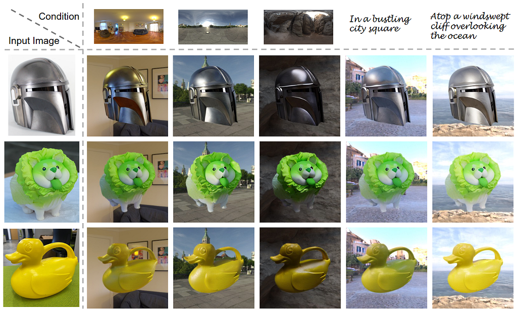
This work proposes an end to end 2D relighting diffusion model. This model learns physical priors from synthetic dataset featuring physically based materials and HDR environment maps. It can be further used to relight multiple views and be used to create a 3D representation of the scene.
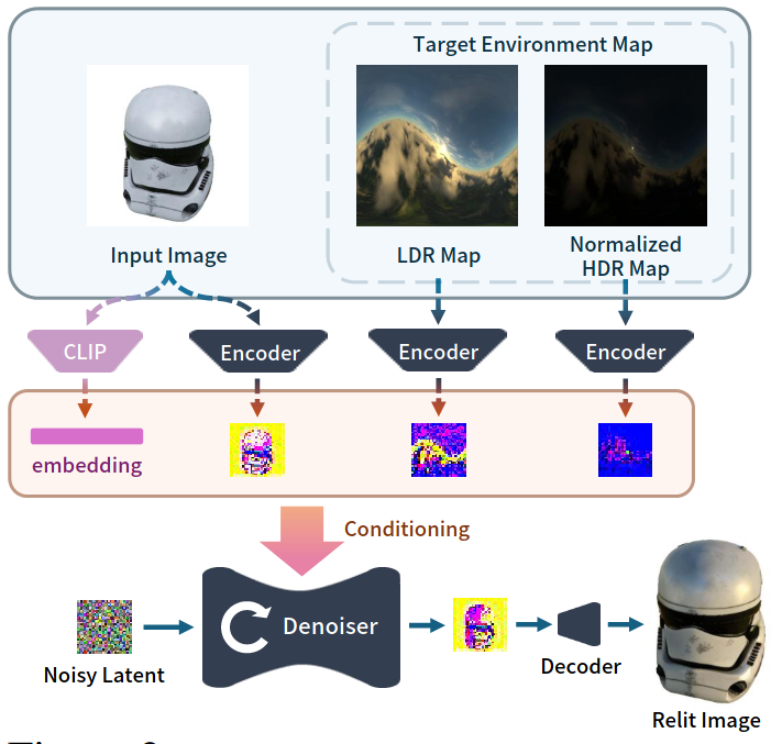
Given an image and a target HDR environment map, the goal is to learn a model that can synthesize a relit version of the image which here is a single object. This is achieved by adopting a pre-trained Zero-1-to-3 model. Zero-1-to-3 is a diffusion model that is conditioned on view direction to render novel views of an input image. They discard its novel view synthesis components. To incorporate lighting conditions, they concatenate input image and environment map encodings with the denoising latent.
The input HDR environment map E is split into two components: E_l, a tone-mapped LDR representation capturing lighting details in low-intensity regions, and E_h, a log-normalized map preserving information across the full spectrum. Together, these provide the network with a balanced representation of the energy spectrum, ensuring accurate relighting without the generated output appearing washed out due to extreme brightness.
Additionally the CLIP embedding of the input image is also passed as input. Thus the input to the model is the Input Image, LDR Image, Normalized HDR Image and CLIP embedding of Image all conditioning the denoising network. This network is then used as prior for further 3D object relighting.
Implementation
The model is trained on a custom Relit Objaverse Dataset that consists of 90K objects. For each object there are 204 images that are rendered under different lighting conditions and viewpoints. In total, the dataset consists of 18.4 M images at resolution 512×512.
The model is finetuned from Zero-1-to-3’s checkpoint and only the denoising network is finetined. The input environment map is downsampled to 256×256 resolution. The model is trained on 8 A6000 GPUs for 5 days. Further downstream tasks such as text-based relighting and object insertion can be achieved.
Results
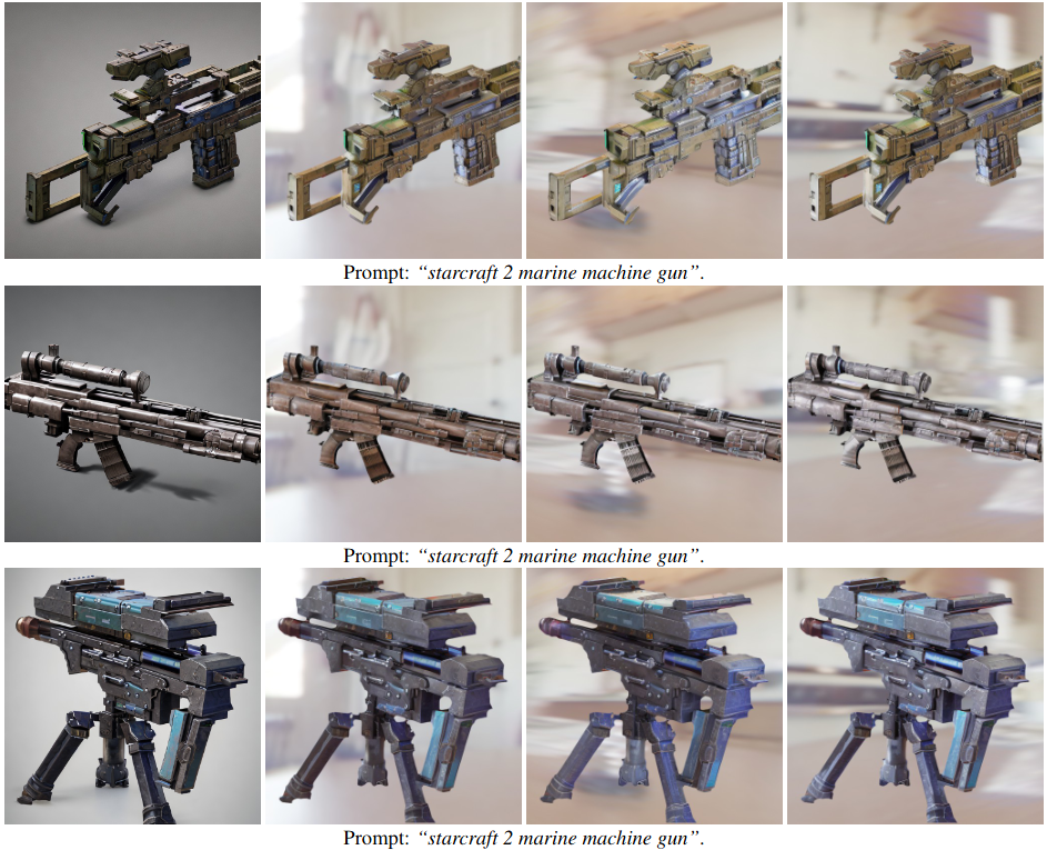
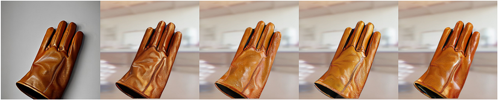
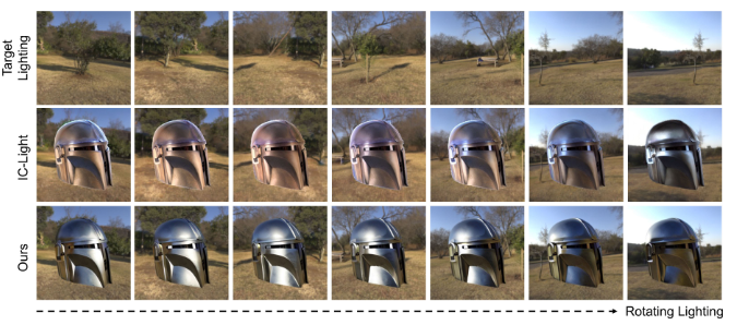
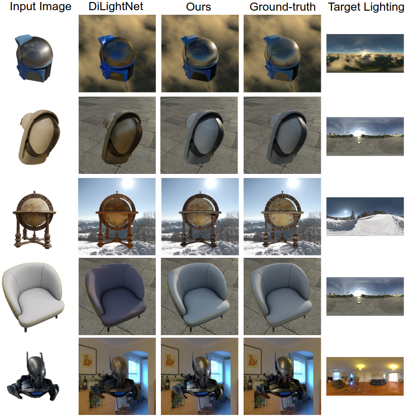
They show comparisons with different backgrounds and comparisons with other works such as DilightNet and IC-Light.
This figure compares the relighting results of their method with IC-Light, another ControlNet based method. Their method can produce consistent lighting and color with the rotating environment map.
This figure compares the relighting results of their method with DiLightnet, another ControlNet based method. Their method can produce specular highlights and accurate colors.
Limitations
A major limitation is that it only produces low image resolution (256×256). Additionally it only works on objects and performs poorly for portrait relighting.
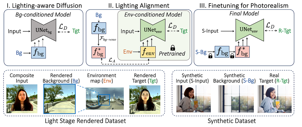
Image Harmonization is the process of aligning the color and lighting features of the foreground subject with the background to make it a plausible composition. This work proposes a diffusion based approach to solve the task.
Given an input composite image, alpha mask and a target background, the goal is to predict a relit portrait image. This is achieved by training a ControlNet to predict the Harmonized image output.
In the first stage, we train a background control net model that takes the composite image and target background as input and outputs a relit portrait image. During training, the denoising network takes the noisy target image concatenated with composite image and predicts the noise. The background is provided as conditioning via the control net. Since background image by itself are LDR, they do not provide sufficient signals for relighting purposes.
In the second stage, an environment map control net model is trained. The HDR environment map provide lot more signals for relighting and this gives lot better results. However at test time, the users only provide LDR backgrounds. Thus, to bridge this gap, the 2 control net models are aligned with each other.
Finally more data is generated using the environment map ControlNet model and then the background ControlNet model is finetuned to generate more photo realistic results.
Implementation
The dataset used for training consists of 400k image pair samples that were curated using 100 lightstage. In the third stage additional 200k synthetic samples were generated for finetuning for photorealism.
The model is finetuned from InstructPix2PIx checkpoint The model is trained on 8 A100 GPUs at 512×512 resolution.
This figure shows how the method neutralizes pronounced shadows in input which are usually hard to remove. On the left is input and right is relit image.
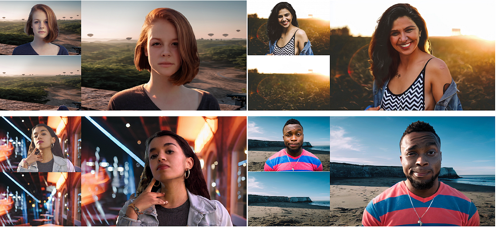
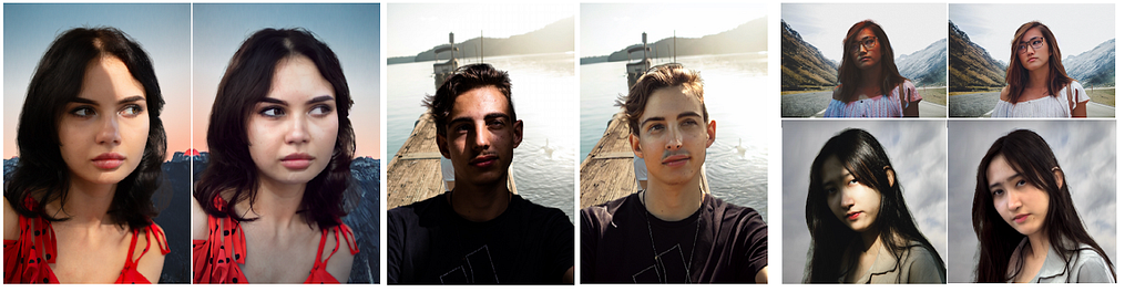
Relightful Harmonization results from sourceRelightful Harmonization results from source
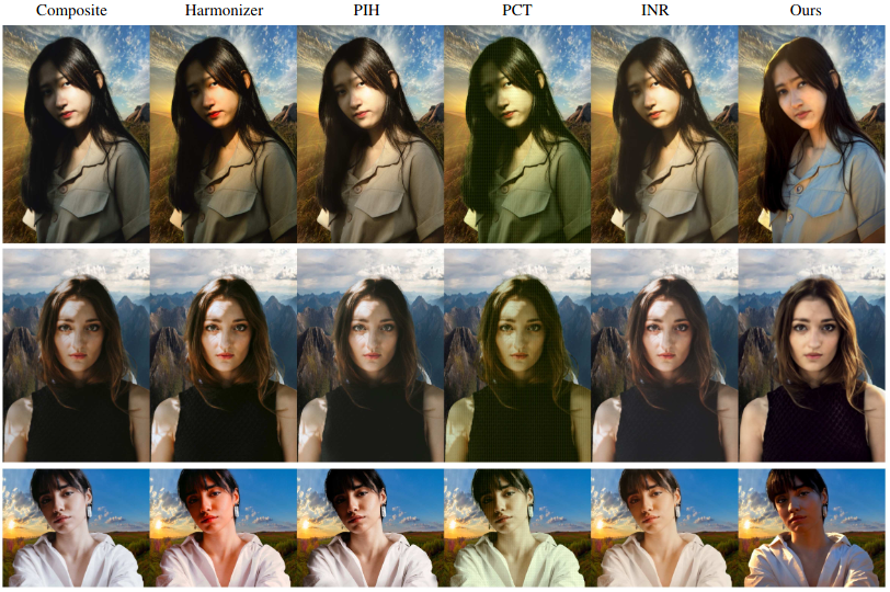
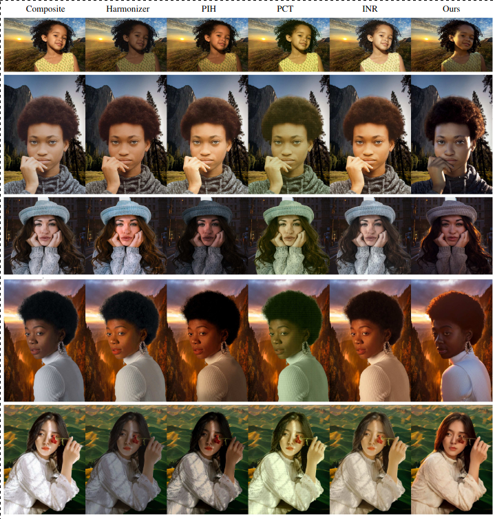
The figures show results on real world test subjects. Their method is able to remove shadows and make the composition more plausible compared to other methods.
Limitations
While this method is able to plausibly relight the subject, it is not great at identity preservation and struggles in maintaining color of the clothes or hair. Further it may struggle to eliminate shadow properly. Also it does not estimate albedo which is crucial for complex light interactions.
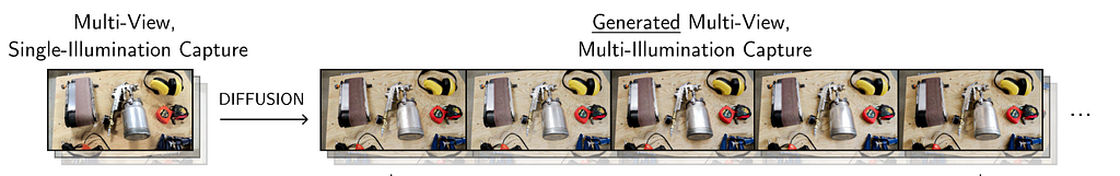
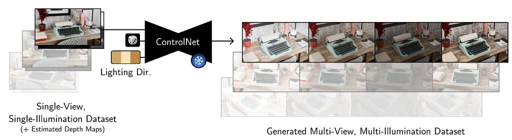
This work proposes a 2D relighting diffusion model that is further used to relight a radiance field of a scene. It first trains a ControlNet model to predict the scene under novel light directions. Then this model is used to generate more data which is eventually used to fit a relightable radiance field. We discuss the 2D relighting model in this section.
Method
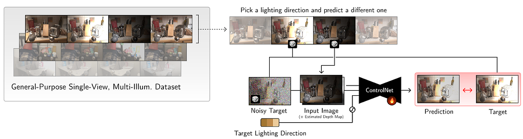
Given a set of images X_i with corresponding depth map D (that is calculated via off the shelf methods), and light direction l_i the goal is to predict the scene under light direction l_j. During training, the input to the denoising network is X_i under random illumination, depth map D concatenated with noisy target image X_j. The light direction is encoded with 4th order SH and conditioned via ControlNet model.
Although this leads to decent results, there are some significant problems. It is unable to preserve colors and leads to loss in contrast. Additionally it produces distorted edges. To resolve this, they color-match the predictions to input image to compensate for color difference. This is done by converting the image to LAB space and then channel normalization. The loss is then taken between ground-truth and denoised output. To preserve edges, the decoder was pretrained on image inpainting tasks which was useful in preserving edges. This network is then used to create corresponding scene under novel light directions which is further used to create a relightable radiance field representation.
Implementation
Inference figure of 2D relighting module from source
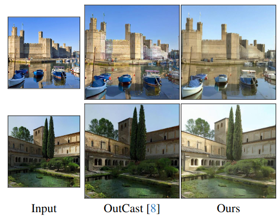
The method was developed upon Multi-Illumination dataset. It consists of 1000 real scenes of indoor scenes captured under 25 lighting directions. The images also consist of a diffuse and a metallic sphere ball that is useful for obtaining the light direction in world coordinates. Additionally some more scenes were rendered in Blender. The network was trained on images at resolution 1536×1024 and training consisted of 18 non-front facing light directions on 1015 indoor scenes.
The ControlNet module was trained using Stable Diffusion v2.1 model as backbone. It was trained on multiple A6000 GPUs for 150K iterations.
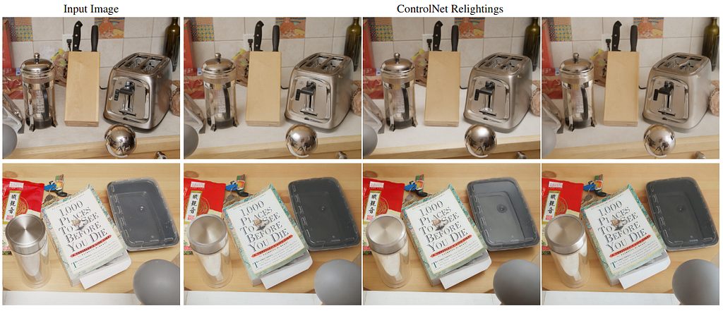
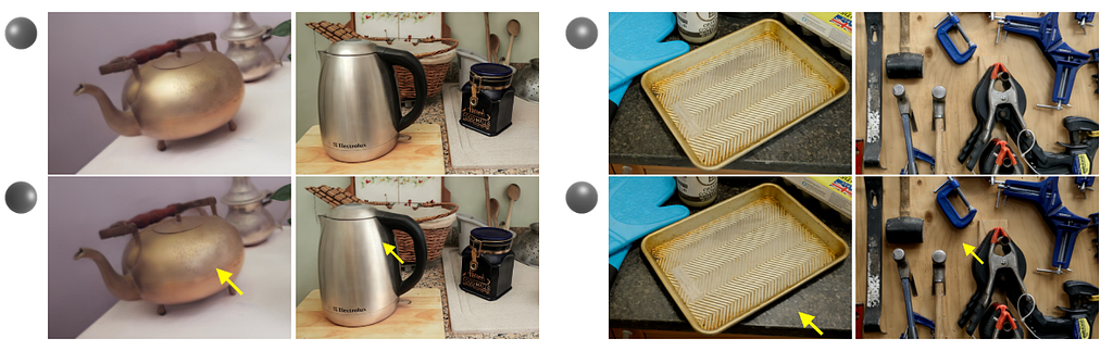
This figure shows how with the changing light direction, the specular highlights and shadows are moving as evident on the shiny highlight on the kettle.
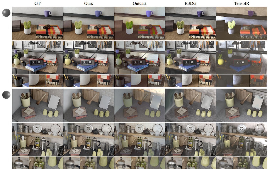
This figure compares results with other relightable radiance field methods. Their method clearly preserves color and contrast much better compared to other methods.
Limitations
The method does not enforce physical accuracy and can produce incorrect shadows. Additionally it also struggles to completely remove shadows in a fully accurate way. Also it does work reasonably for out of distribution scenes where the variance in lighting is not much.
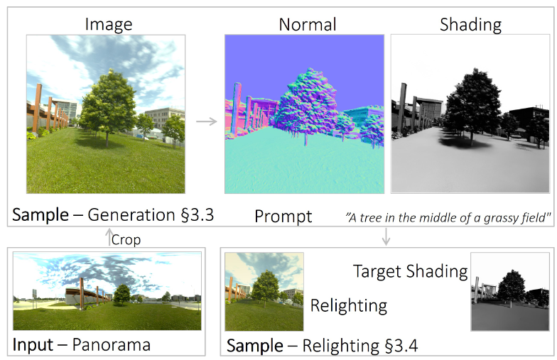
This work proposes a single view shading estimation method to generate a paired image and its corresponding direct light shading. This shading can then be used to guide the generation of the scene and relight a scene. They approach the problem as an intrinsic decomposition problem where the scene can be split into Reflectance and Shading. We will discuss the relighting component here.
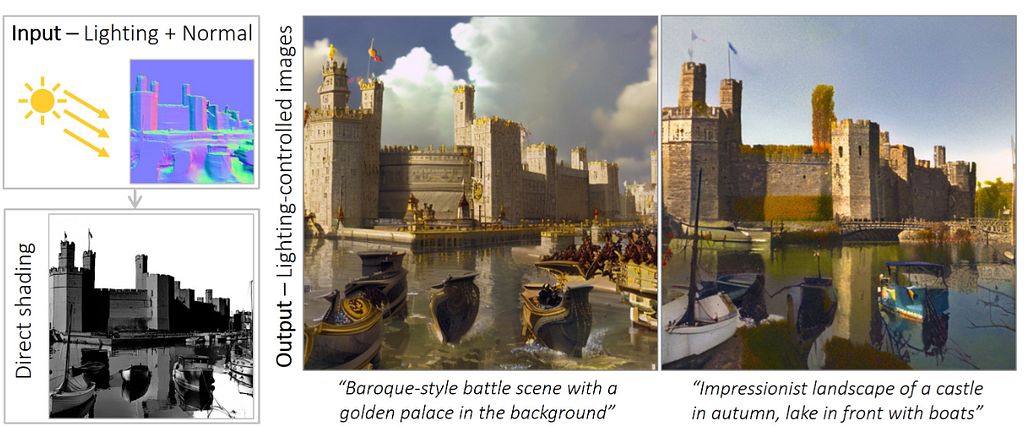
Given an input image, its corresponding surface normal, text conditioning and a target direct shading image, they generate a relit stylized image. This is achieved by training a ControlNet module.
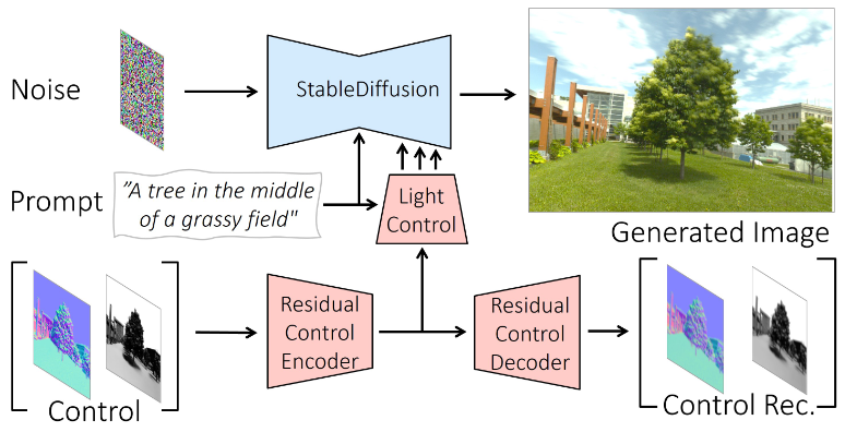
During training, the noisy target image is passed to the denoising network along with text conditioning. The normal and target direct shading image are concatenated and passed through a Residual Control Encoder. The feature map is then used to condition the network. Additionally its also reconstructed back via Residual Control Decoder to regularize the training
The dataset consists of Outdoor Laval Dataset which consist of outdoor real world HDR panoramas. From these images, 250 512×512 images are cropped and various camera effects are applied. The dataset consists of 51250 samples of LDR images and text prompts along with estimated normal and shading maps. The normals maps were estimated from depth maps that were estimated using off the shelf estimators.
The ControlNet module was finetuned from stable diffusion v1.5. The network was trained for two epochs. Other training details are not shared.
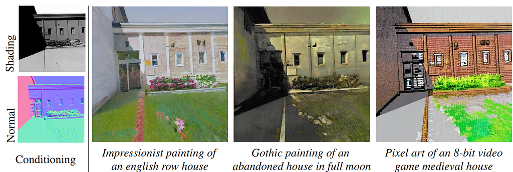
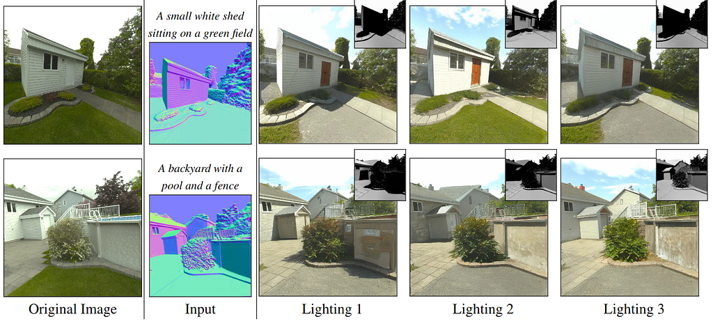
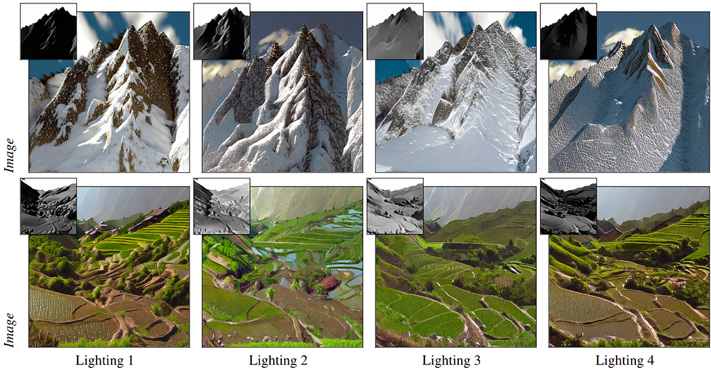
This figure shows that the generated images feature consistent lighting aligned with target shading for custom stylized text prompts. This is different from other papers discussed whose sole focus is on photorealism.
This figure compares relighting with another method. Utilizing the diffusion prior helps with generalization and resolving shading disambiguation.
Limitations
Since this method assumes directional lighting, it enables tracing rays in arbitrary direction. It requires shading cues to generate images which are non trivial to obtain. Further their method does not work for portraits and indoor scenes.
Takeaways
We have discussed a non-exhaustive list of papers that leverage 2D diffusion models for relighting purposes. We explored different ways to condition Diffusion models for relighting ranging from radiance cues, direct shading images, light directions and environment maps. Most of these methods show results on synthetic datasets and dont generalize well to out of distribution datasets. There are more papers coming everyday and the base models are also improving. Recently IC-Light2 was released which is a ControlNet model based upon Flux models. It will be interesting which direction it takes as maintaining identities is tricky.
Getting your AI task to distinguish between Hard and Easy problems
In this position paper, I discuss the premise that a lot of potential performance enhancement is left on the table because we don’t often address the potential of dynamic execution.
I guess I need to first define what is dynamic execution in this context. As many of you are no doubt aware of, we often address performance optimizations by taking a good look at the model itself and what can be done to make processing of this model more efficient (which can be measured in terms of lower latency, higher throughput and/or energy savings).
These methods often address the size of the model, so we look for ways to compress the model. If the model is smaller, then memory footprint and bandwidth requirements are improved. Some methods also address sparsity within the model, thus avoiding inconsequential calculations.
Still… we are only looking at the model itself.
This is definitely something we want to do, but are there additional opportunities we can leverage to boost performance even more? Often, we overlook the most human-intuitive methods that don’t focus on the model size.
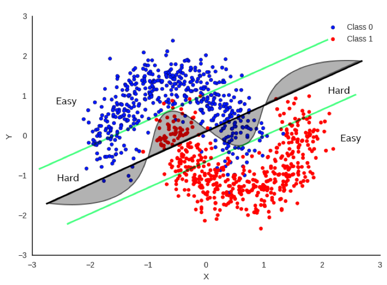
Figure 1. Intuition of hard vs easy decisions
Hard vs Easy
In Figure 1, there’s a simple example (perhaps a bit simplistic) regarding how to classify between red and blue data points. It would be really useful to be able to draw a decision boundary so that we know the red and blue points are on opposite sides of the boundary as much as possible. One method is to do a linear regression whereby we fit a straight line as best as we can to separate the data points as much as possible. The bold black line in Figure 1 represents one potential boundary. Focusing only on the bold black line, you can see that there is a substantial number of points that fall on the wrong side of the boundary, but it does a decent job most of the time.
If we focus on the curved line, this does a much better job, but it’s also more difficult to compute as it’s no longer a simple, linear equation. If we want more accuracy, clearly the curve is a much better decision boundary than the black line.
But let’s not just throw out the black line just yet. Now let’s look at the green parallel lines on each side of the black boundary. Note that the linear decision boundary is very accurate for points outside of the green line. Let’s call these points “Easy”.
In fact, it is 100% as accurate as the curved boundary for Easy points. Points that lie inside the green lines are “Hard” and there is a clear advantage to using the more complex decision boundary for these points.
So… if we can tell if the input data is hard or easy, we can apply different methods to solving the problem with no loss of accuracy and a clear savings of computations for the easy points.
This is very intuitive as this is exactly how humans address problems. If we perceive a problem as easy, we often don’t think too hard about it and give an answer quickly. If we perceive a problem as being hard, we think more about it and often it takes more time to get to the answer.
So, can we apply a similar approach to AI?
Dynamic Execution Methods
In the dynamic execution scenario, we employ a set of specialized techniques designed to scrutinize the specific query at hand. These techniques involve a thorough examination of the query’s structure, content, and context with the aim of discerning whether the problem it represents can be addressed in a more straightforward manner.
This approach mirrors the way humans tackle problem-solving. Just as we, as humans, are often able to identify problems that are ’easy’ or ’simple’ and solve them with less effort compared to ’hard’ or ’complex’ problems, these techniques strive to do the same. They are designed to recognize simpler problems and solve them more efficiently, thereby saving computational resources and time.
This is why we refer to these techniques as Dynamic Execution. The term ’dynamic’ signifies the adaptability and flexibility of this approach. Unlike static methods that rigidly adhere to a predetermined path regardless of the problem’s nature, Dynamic Execution adjusts its strategy based on the specific problem it encounters, that is, the opportunity is data dependent.
The goal of Dynamic Execution is not to optimize the model itself, but to optimize the compute flow. In other words, it seeks to streamline the process through which the model interacts with the data. By tailoring the compute flow to the data presented to the model, Dynamic Execution ensures that the model’s computational resources are utilized in the most efficient manner possible.
In essence, Dynamic Execution is about making the problem-solving process as efficient and effective as possible by adapting the strategy to the problem at hand, much like how humans approach problem-solving. It is about working smarter, not harder. This approach not only saves computational resources but also improves the speed and accuracy of the problem-solving process.
Early Exit
This technique involves adding exits at various stages in a deep neural network (DNN). The idea is to allow the network to terminate the inference process earlier for simpler tasks, thus saving computational resources. It takes advantage of the observation that some test examples can be easier to predict than others [1], [2].
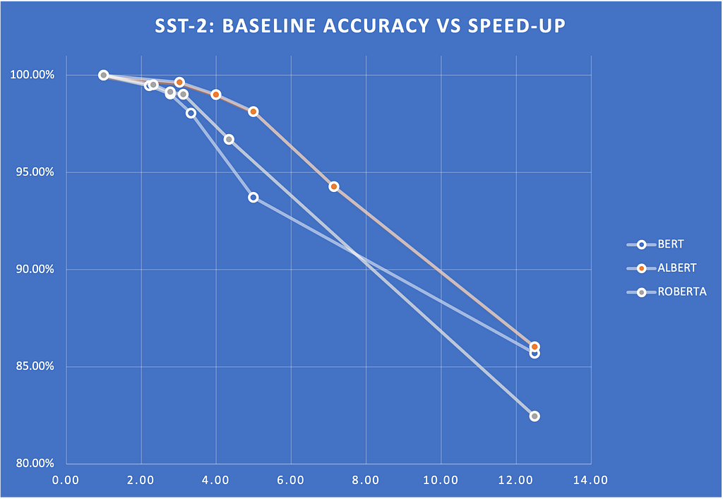
Below is an example of the Early Exit strategy in several encoder models, including BERT, ROBERTA, and ALBERT.
We measured the speed-ups on glue scores for various entropy thresholds. Figure 2 shows a plot of these scores and how they drop with respect to the entropy threshold. The scores show the percentage of the baseline score (that is, without Early Exit). Note that we can get 2x to 4X speed-up without sacrificing much quality.
Figure 2. Early Exit: SST-2
Speculative Sampling
This method aims to speed up the inference process by computing several candidate tokens from a smaller draft model. These candidate tokens are then evaluated in parallel in the full target model [3], [4].
Speculative sampling is a technique designed to accelerate the decoding process of large language models [5], [6]. The concept behind speculative sampling is based on the observation that the latency of parallel scoring of short continuations, generated by a faster but less powerful draft model, is comparable to that of sampling a single token from the larger target model. This approach allows multiple tokens to be generated from each transformer call, increasing the speed of the decoding process.
The process of speculative sampling involves two models: a smaller, faster draft model and a larger, slower target model. The draft model speculates what the output is several steps into the future, while the target model determines how many of those tokens we should accept. The draft model decodes several tokens in a regular autoregressive fashion, and the probability outputs of the target and the draft models on the new predicted sequence are compared. Based on some rejection criteria, it is determined how many of the speculated tokens we want to keep. If a token is rejected, it is resampled using a combination of the two distributions, and no more tokens are accepted. If all speculated tokens are accepted, an additional final token can be sampled from the target model probability output.
In terms of performance boost, speculative sampling has shown significant improvements. For instance, it was benchmarked with Chinchilla, a 70 billion parameter language model, achieving a 2–2.5x decoding speedup in a distributed setup, without compromising the sample quality or making modifications to the model itself. Another example is the application of speculative decoding to Whisper, a general purpose speech transcription model, which resulted in a 2x speed-up in inference throughput [7], [8]. Note that speculative sampling can be used to boost CPU inference performance, but the boost will likely be less (typically around 1.5x).
In conclusion, speculative sampling is a promising technique that leverages the strengths of both a draft and a target model to accelerate the decoding process of large language models. It offers a significant performance boost, making it a valuable tool in the field of natural language processing. However, it is important to note that the actual performance boost can vary depending on the specific models and setup used.
StepSaver
This is a method that could also be called Early Stopping for Diffusion Generation, using an innovative NLP model specifically fine-tuned to determine the minimal number of denoising steps required for any given text prompt. This advanced model serves as a real-time tool that recommends the ideal number of denoising steps for generating high-quality images efficiently. It is designed to work seamlessly with the Diffusion model, ensuring that images are produced with superior quality in the shortest possible time. [9]
Diffusion models iteratively enhance a random noise signal until it closely resembles the target data distribution [10]. When generating visual content such as images or videos, diffusion models have demonstrated significant realism [11]. For example, video diffusion models and SinFusion represent instances of diffusion models utilized in video synthesis [12][13]. More recently, there has been growing attention towards models like OpenAI’s Sora; however, this model is currently not publicly available due to its proprietary nature.
Performance in diffusion models involves a large number of iterations to recover images or videos from Gaussian noise [14]. This process is called denoising and is trained on a specific number of iterations of denoising. The number of iterations in this sampling procedure is a key factor in the quality of the generated data, as measured by metrics, such as FID.
Latent space diffusion inference uses iterations in feature space, and performance suffers from the expense of many iterations required for quality output. Various techniques, such as patching transformation and transformer-based diffusion models [15], improve the efficiency of each iteration.
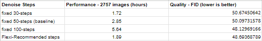
StepSaver dynamically recommends significantly lower denoising steps, which is critical to address the slow sampling issue of stable diffusion models during image generation [9]. The recommended steps also ensure better image quality. Figure 3 shows that images generated using dynamic steps result in a 3X throughput improvement and a similar image quality compared to static 100 steps.
Figure 3. StepSaver Performance
LLM Routing
Dynamic Execution isn’t limited to just optimizing a specific task (e.g. generating a sequence of text). We can take a step above the LLM and look at the entire pipeline. Suppose we are running a huge LLM in our data center (or we’re being billed by OpenAI for token generation via their API), can we optimize the calls to LLM so that we select the best LLM for the job (and “best” could be a function of token generation cost). Complicated prompts might require a more expensive LLM, but many prompts can be handled with much lower cost on a simpler LLM (or even locally on your notebook). So if we can route our prompt to the appropriate destination, then we can optimize our tasks based on several criteria.
Routing is a form of classification in which the prompt is used to determine the best model. The prompt is then routed to this model. By best, we can use different criteria to determine the most effective model in terms of cost and accuracy. In many ways, routing is a form of dynamic execution done at the pipeline level where many of the other optimizations we are focusing on in this paper is done to make each LLM more efficient. For example, RouteLLM is an open-source framework for serving LLM routers and provides several mechanisms for reference, such as matrix factorization. [16] In this study, the researchers at LMSys were able to save 85% of costs while still keeping 95% accuracy.
Conclusion
This certainly was not meant to be an exhaustive study of all dynamic execution methods, but it should provide data scientists and engineers with the motivation to find additional performance boosts and cost savings from the characteristics of the data and not solely focus on model-based methods. Dynamic Execution provides this opportunity and does not interfere with or hamper traditional model-based optimization efforts.
Unless otherwise noted, all images are by the author.
[1] K. Liao, Y. Zhang, X. Ren, Q. Su, X. Sun, and B. He, “A Global Past-Future Early Exit Method for Accelerating Inference of Pre-trained Language Models,” in Conference of the North American Chapter of the Association for Computational Linguistics: Human Language Technologies, pp. 2013–2023, Association for Computational Linguistics (ACL), June 2021.
[2] F. Ilhan, K.-H. Chow, S. Hu, T. Huang, S. Tekin, W. Wei, Y. Wu, M. Lee, R. Kompella, H. Latapie, G. Liu, and L. Liu, “Adaptive Deep Neural Network Inference Optimization with EENet,” Dec. 2023. arXiv:2301.07099 [cs].
[3] Y. Leviathan, M. Kalman, and Y. Matias, “Fast Inference from Transformers via Speculative Decoding,” May 2023. arXiv:2211.17192 [cs].
[4] H. Barad, E. Aidova, and Y. Gorbachev, “Leveraging Speculative Sampling and KV-Cache Optimizations Together for Generative AI using OpenVINO,” Nov. 2023. arXiv:2311.04951 [cs].
[5] C. Chen, S. Borgeaud, G. Irving, J.-B. Lespiau, L. Sifre, and J. Jumper, “Accelerating Large Language Model Decoding with Speculative Sampling,” Feb. 2023. arXiv:2302.01318 [cs] version: 1.
[6] J. Mody, “Speculative Sampling,” Feb. 2023.
[7] J. Gante, “Assisted Generation: a new direction toward low-latency text generation,” May 2023.
[8] S. Gandhi, “Speculative Decoding for 2x Faster Whisper Inference.”
[9] J. Yu and H. Barad, “Step Saver: Predicting Minimum Denoising Steps for Diffusion Model Image Generation,” Aug. 2024. arXiv:2408.02054 [cs].
[10] Notomoro, “Diffusion Model: A Comprehensive Guide With Example,” Feb. 2024. Section: Artificial Intelligence.
[11] T. H¨oppe, A. Mehrjou, S. Bauer, D. Nielsen, and A. Dittadi, “Diffusion Models for Video Prediction and Infilling,” Nov. 2022. arXiv:2206.07696 [cs, stat].
[12] J. Ho, T. Salimans, A. Gritsenko, W. Chan, M. Norouzi, and D. J. Fleet, “Video Diffusion Models,” June 2022. arXiv:2204.03458 [cs].
[13] Y. Nikankin, N. Haim, and M. Irani, “SinFusion: Training Diffusion Models on a Single Image or Video,” June 2023. arXiv:2211.11743 [cs].
[14] Z. Chen, Y. Zhang, D. Liu, B. Xia, J. Gu, L. Kong, and X. Yuan, “Hierarchical Integration Diffusion Model for Realistic Image Deblurring,” Sept. 2023. arXiv:2305.12966 [cs]
[15] W. Peebles and S. Xie, “Scalable Diffusion Models with Transformers,” Mar. 2023. arXiv:2212.09748 [cs].
[16] I. Ong, A. Almahairi, V. Wu, W.-L. Chiang, T. Wu, J. E. Gonzalez, M. W. Kadous, and I. Stoica, “RouteLLM: Learning to Route LLMs with Preference Data,” July 2024. arXiv:2406.18665 [cs].
Dynamic Execution was originally published in Towards Data Science on Medium, where people are continuing the conversation by highlighting and responding to this story.
Antitrust regulators in the European Union are set to judge whether or not Apple has done enough to bring its iPad operating system under compliance with rules outlined in the Digital Markets Act.
iPadOS
In March, Apple released iPadOS 17.4, with more than 600 new APIs, expanded app analytics, functionality for alternative browser engines, and more. The changes allowed third-party developers to distribute apps outside of Apple’s App Store in the EU, a change Apple begrudgingly made to comply with the Digital Markets App (DMA).
Now, EU regulators are assessing whether or not Apple has gone far enough. The assessment will be based on the input of interested stakeholders.
Thunderbolt 5 has arrived, and Apple has adopted it on some of its new Mac models. Here’s what has changed in Thunderbolt 5 vs. Thunderbolt 4.
Thunderbolt 5 vs Thunderbolt 4 — USB Type-C continues to be used.
As a connectivity technology, Thunderbolt is deeply associated with Apple, due to its usage in Macs and then, later, the iPad Pro. Many of its products now support Thunderbolt 4, with it providing massive amounts of bandwidth for data transfers, as well as handling charging and even video duties.
Just like many other standards in the tech world, Thunderbolt is iteratively upgraded over time with new features. While the world is largely on Thunderbolt 4 for the moment, Thunderbolt 5 is just starting its rollout, and it promises to make big changes to what it can offer to users.
On this episode of the HomeKit Insider Podcast we talk about Apple’s continued use of hidden Thread radios, Apple TV’s new watch list feature, and more new smart home products launching.
HomeKit Insider Podcast
Recently, Apple launched tvOS 18.1 which didn’t contain many user-facing feature. One seems to have flown under the radar though.
With this update, the TV app has a new separate watch list for movies and TV shows that you have not started. This differs from the Up Next queue that shows all content — stuff you’ve started watching and stuff you have not.
Your iPhone’s next iOS 18.2 update may come earlier than usual – with these AI features
Originally appeared here:
Your iPhone’s next iOS 18.2 update may come earlier than usual – with these AI features
We use cookies on our website to give you the most relevant experience by remembering your preferences and repeat visits. By clicking “Accept”, you consent to the use of ALL the cookies.
This website uses cookies to improve your experience while you navigate through the website. Out of these, the cookies that are categorized as necessary are stored on your browser as they are essential for the working of basic functionalities of the website. We also use third-party cookies that help us analyze and understand how you use this website. These cookies will be stored in your browser only with your consent. You also have the option to opt-out of these cookies. But opting out of some of these cookies may affect your browsing experience.
Necessary cookies are absolutely essential for the website to function properly. These cookies ensure basic functionalities and security features of the website, anonymously.
Cookie
Duration
Description
cookielawinfo-checkbox-analytics
11 months
This cookie is set by GDPR Cookie Consent plugin. The cookie is used to store the user consent for the cookies in the category "Analytics".
cookielawinfo-checkbox-functional
11 months
The cookie is set by GDPR cookie consent to record the user consent for the cookies in the category "Functional".
cookielawinfo-checkbox-necessary
11 months
This cookie is set by GDPR Cookie Consent plugin. The cookies is used to store the user consent for the cookies in the category "Necessary".
cookielawinfo-checkbox-others
11 months
This cookie is set by GDPR Cookie Consent plugin. The cookie is used to store the user consent for the cookies in the category "Other.
cookielawinfo-checkbox-performance
11 months
This cookie is set by GDPR Cookie Consent plugin. The cookie is used to store the user consent for the cookies in the category "Performance".
viewed_cookie_policy
11 months
The cookie is set by the GDPR Cookie Consent plugin and is used to store whether or not user has consented to the use of cookies. It does not store any personal data.
Functional cookies help to perform certain functionalities like sharing the content of the website on social media platforms, collect feedbacks, and other third-party features.
Performance cookies are used to understand and analyze the key performance indexes of the website which helps in delivering a better user experience for the visitors.
Analytical cookies are used to understand how visitors interact with the website. These cookies help provide information on metrics the number of visitors, bounce rate, traffic source, etc.
Advertisement cookies are used to provide visitors with relevant ads and marketing campaigns. These cookies track visitors across websites and collect information to provide customized ads.