Overcoming Outliers with ROBPCA

A Guide to Hubert et al.’s Robust PCA Procedure (ROBPCA)

Principal components analysis is a variance decomposition technique that is frequently used for dimensionality reduction. A thorough guide to PCA is available here. In essence, each principal component is computed by finding the linear combination of the original features which has maximal variance, subject to the constraint that it must be orthogonal to the previous principal components. This process tends to be sensitive to outliers as it does not differentiate between meaningful variation and variance due to noise. The top principal components, which represent the directions of maximum variance, are especially susceptible.

In this article, I will discuss ROBPCA, a robust alternative to classical PCA which is less sensitive to extreme values. I will explain the steps of the ROBPCA procedure, discuss how to implement it with the R package ROSPCA, and illustrate its use on the wine quality dataset from the UCI Machine Learning Repository. To conclude, I will consider some limitations of ROBPCA and discuss an alternative robust PCA algorithm which is noteworthy but not well-suited for this particular dataset.

ROBPCA Procedure:

The paper which proposed ROBPCA was published in 2005 by Belgian statistician Mia Hubert and colleagues. It has garnered thousands of citations, including hundreds within the past couple of years, but the procedure is not often covered in data science courses and tutorials. Below, I’ve described the steps of the algorithm:

I) Center the data using the usual estimator of the mean, and perform a singular value decomposition (SVD). This step is particularly helpful when p>n or the covariance matrix is low-rank. The new data matrix is taken to be UD, where U is an orthogonal matrix whose columns are the left singular vectors of the data matrix, and D is the diagonal matrix of singular values.

II) Identify a subset of h_0 ‘least outlying’ data points, drawing on ideas from projection pursuit, and use these core data points to determine how many robust principal components to retain. This can be broken down into three sub-steps:

a) Project each data point in several univariate directions. For each direction, determine how extreme each data point is by standardizing with respect to the maximum covariance determinant (MCD) estimates of the location and scatter. In this case, the MCD estimates are the mean and the standard deviation of the h_0 data points with the smallest variance when projected in the given direction.

b) Retain the subset of h_0 data points which have the smallest maximum standardized score across all of the different directions considered in the previous sub-step.

c) Compute a covariance matrix S_0 from the h_0 data points and use S_0 to select k, the number of robust principal components. Project the full dataset onto the top k eigenvectors of S_0.

III) Robustly calculate the scatter of the final data from step two using an accelerated MCD procedure. This procedure finds a subset of h_1 data points with minimal covariance determinant from the subset of h_0 data points identified previously. The top k eigenvectors of this scatter matrix are taken to be the robust principal components. (In the event that the accelerated MCD procedure leads to a singular matrix, the data is projected onto a lower-dimensional space, ultimately resulting in fewer than k robust principal components.)

Note that classical PCA can be expressed in terms of the same SVD that is used in step one of ROBPCA; however, ROBPCA involves additional steps to limit the influence of extreme values, while classical PCA immediately retains the top k principal components.

ROSPCA Package:

ROBPCA was initially implemented in the rrcov package via the PcaHubert function, but a more efficient implementation is now available in the ROSPCA package. This package contains additional methods for robust sparse PCA, but these are beyond the scope of this article. I will illustrate the use of the robpca function, which depends on two important parameters: alpha and k. Alpha controls how many outlying data points are resisted, taking on values in the range [0.5, 1.0]. The relationship between h_0 and alpha is given by:

The parameter k determines how many robust principal components to retain. If k is not specified, it is chosen as the smallest number such that a) the eigenvalues satisfy:

and b) the retained principal components explain at least 80 percent of the variance among the h_0 least outlying data points. When no value of k satisfies both criteria, then just the ratio of the eigenvalues is used to determine how many principal components will be retained. (Note: the original PcaHubert function states the criterion as 10E-3, but the robpca function uses 1E-3.)

Real Data Example:

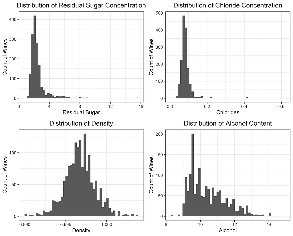
For this case study, I have selected the red wine quality dataset from the UCI Machine Learning Repository. The dataset contains n=1,599 observations, each representing a different red wine. The 12 variables include 11 different chemical properties and an expert quality rating. Several of the 11 chemical properties contain potential outliers, making this an ideal dataset to illustrate 1) the impact of extreme values on PCA and 2) how a robust variance structure can be identified through ROBPCA.

PCA is not scale-invariant, so it’s important to decide intentionally on what, if any, standardization will be used. Failing to standardize would give undue weight to variables measured on larger scales, so I center each of the 11 features and divide by its standard deviation. An alternative approach would be to use a robust measure of center and scale such as the median and MAD; however, I find that robust estimates of the scale completely distort the classical principal components since the extreme values are even farther from the data’s center. ROBPCA is less sensitive to the initial scaling (a considerable advantage in itself), but I use the standard deviation for consistency and to ensure the results are comparable.

To select k for ROBPCA, I allow the function to determine the optimal k value, resulting in k=5 robust principal components. I accept the default of alpha=0.75 since I find that the variable loadings are not very sensitive to the choice of alpha, with alpha values between 0.6 and 0.9 producing very similar loadings. For classical PCA, I let k=5 to facilitate comparisons between the two methods. This is a reasonable choice for classical PCA, irrespective of ROBPCA, as the top five principal components explain just under 80 percent of the total variance.

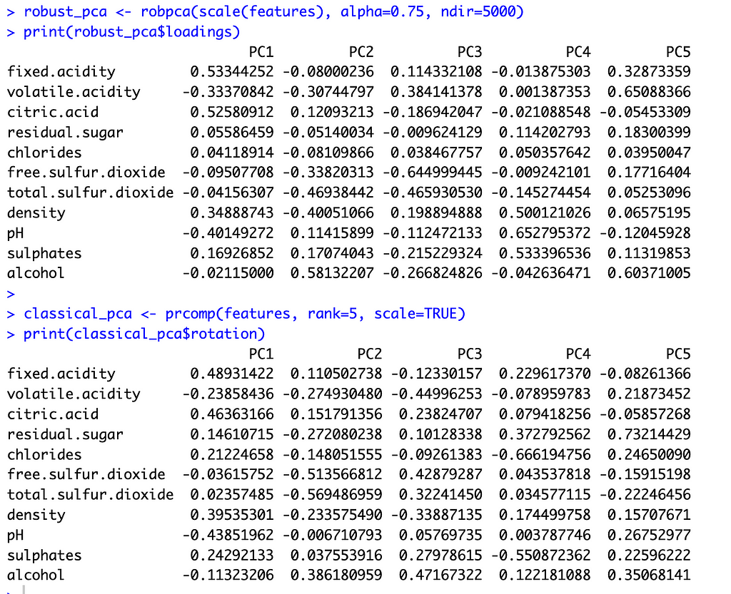
With these preliminaries out of the way, let’s compare the two methods. The image below shows the principal component loadings for both methods. Across all five components, the loadings on the variables ‘residual sugar’ and ‘chlorides’ are much smaller (in absolute value) for ROBPCA than for classical PCA. Both of these variables contain a large number of outliers, which ROBPCA tends to resist.

Meanwhile, the variables ‘density’ and ‘alcohol’ seem to contribute more significantly to the robust principal components. The second robust component, for instance, has much larger loadings on these variables than does the second classical component. The fourth and fifth robust components also have much larger loadings on either ‘density’ or ‘alcohol,’ respectively, than their classical counterparts. There are few outliers in terms of density and alcohol content, with almost all red wines distributed along a continuum of values. ROBPCA seems to better capture these common sources of variation.

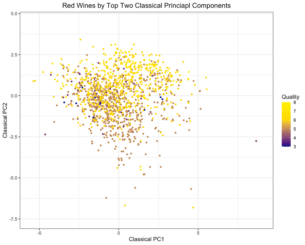
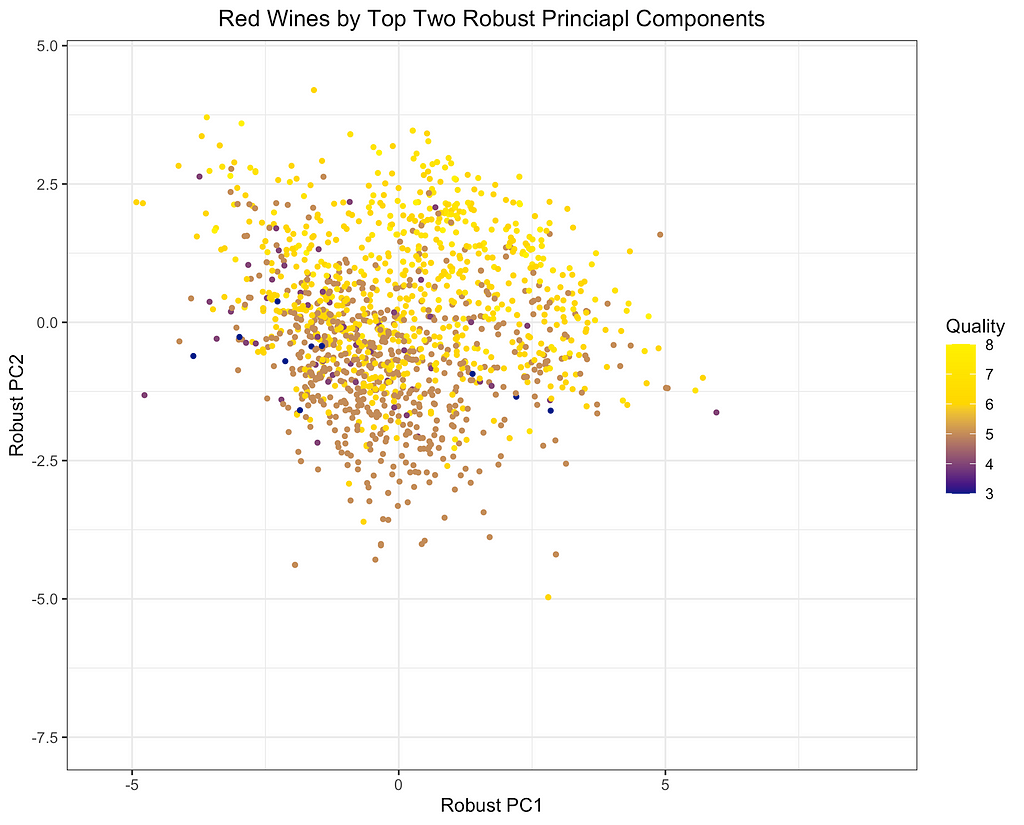
Finally, I will depict the differences between ROBPCA and classical PCA by plotting the scores for the top two principal components against each other, a common technique used for visualizing datasets in a low-dimensional space. As can be seen from the first plot below, there are a number of outliers in terms of the classical principal components, most of which have a large negative loading on PC1 and/or a large positive loading on PC2. There are a few potential outliers in terms of the robust principal components, but they do not deviate as much from the main cluster of data points. The differences between the two plots, particularly in the upper left corner, indicate that the classical principal components may be skewed downward in the direction of the outliers. Moreover, it appears that the robust principal components can better separate the wines by quality, which was not used in the principal components decomposition, providing some indication that ROBPCA recovers more meaningful variation in the data.

This example demonstrates how ROBPCA can resist extreme values and identify sources of variation that better represent the majority of the data points. However, the choice between robust PCA and classical PCA will ultimately depend on the dataset and the objective of the analysis. Robust PCA has the greatest advantage when there are extreme values due to measurement errors or other sources of noise that are not meaningfully related to the phenomenon of interest. Classical PCA is often preferred when the extreme values represent valid measurements, but this will depend on the objective of the analysis. Regardless of the validity of the outliers, I’ve found that robust PCA can have a large advantage when the objective of the analysis is to cluster the data points and/or visualize their distribution using only the top two or three components. The top components are especially susceptible to outliers, and they may not be very useful for segmenting the majority of data points when extreme values are present.

Potential Limitations of ROBPCA Procedure:

While ROBPCA is a powerful tool, there are some limitations of which the reader should be aware:

1. The projection procedure in step two can be time consuming. If n>500, the ROSPCA package recommends setting the maximum number of directions to 5,000. Even fixing ndir=5,000, the projection step still has time complexity O(np + nlog(n)), where the nlog(n) term is the time complexity for finding the MCD estimates of location and scale. This might be unsuitable for very large n and/or p.
2. The robust principal components are not an orthogonal basis for the full dataset, which includes the outlying data points that were resisted in the identification of the robust components. If uncorrelated predictors are desired, then ROBPCA might not be the best approach.

An Alternative Robust PCA Algorithm:

There are various alternative approaches to robust PCA, including a method proposed by Candes et al. (2011), which seeks to decompose the data matrix into a low-dimensional component and a sparse component. This approach is implemented in the rpca R package. I applied this method on the red wine dataset, but over 80 percent of the entries in the sparse matrix were non-zero. This low sparsity level indicates that the assumptions of the method were not well met. While this alternative approach is not very suitable for the red wine data, it could be a very useful algorithm for other datasets where the assumed decomposition is more appropriate.

References:

M. Hubert, P. J. Rousseeuw, K. Vanden Branden, ROBPCA: a new approach to robust principal components analysis (2005), Technometrics.

E. Candes, X. Li, Y. Ma, J. Wright, Robust Principal Components Analysis? (2011), Journal of the ACM (JACM).

T. Reynkens, V. Todorov, M. Hubert, E. Schmitt, T. Verdonck, rospca: Robust Sparse PCA using the ROSPCA Algorithm (2024), Comprehensive R Archive Network (CRAN).

V. Todorov, rrcov: Scalable Robust Estimators with High Breakdown Point (2024), Comprehensive R Archive Network (CRAN).

M. Sykulski, rpca: RobustPCA: Decompose a Matrix into Low-Rank and Sparse Components (2015), Comprehensive R Archive Network (CRAN).

P. Cortez, A. Cerdeira, F. Almeida, T. Matos, J. Reis, Wine Quality (2009), UC Irvine Machine Learning Repository. (CC BY 4.0)

Overcoming Outliers with ROBPCA was originally published in Towards Data Science on Medium, where people are continuing the conversation by highlighting and responding to this story.