Monocular Depth Estimation with Depth Anything V2

How do neural networks learn to estimate depth from 2D images?

What is Monocular Depth Estimation?

Monocular Depth Estimation (MDE) is the task of training a neural network to determine depth information from a single image. This is an exciting and challenging area of Machine Learning and Computer Vision because predicting a depth map requires the neural network to form a 3-dimensional understanding from just a 2-dimensional image.

In this article, we will discuss a new model called Depth Anything V2 and its precursor, Depth Anything V1. Depth Anything V2 has outperformed nearly all other models in Depth Estimation, showing impressive results on tricky images.

This article is based on a video I made on the same topic. Here is a video link for learners who prefer a visual medium. For those who prefer reading, continue!

Why should we even care about MDE models?

Good MDE models have many practical uses, such as aiding navigation and obstacle avoidance for robots, drones, and autonomous vehicles. They can also be used in video and image editing, background replacement, object removal, and creating 3D effects. Additionally, they are useful for AR and VR headsets to create interactive 3D spaces around the user.

There are two main approaches for doing MDE (this article only covers one)

Two main approaches have emerged for training MDE models — one, discriminative approaches where the network tries to predict depth as a supervised learning objective, and two, generative approaches like conditional diffusion where depth prediction is an iterative image generation task. Depth Anything belongs to the first category of discriminative approaches, and that’s what we will be discussing today. Welcome to Neural Breakdown, and let’s go deep with Depth Estimation[!

Traditional Datasets and the MiDAS paper

To fully understand Depth Anything, let’s first revisit the MiDAS paper from 2019, which serves as a precursor to the Depth Anything algorithm.

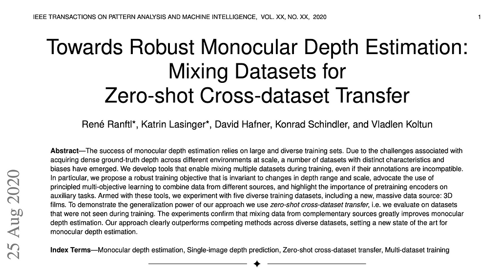
MiDAS trains an MDE model using a combination of different datasets containing labeled depth information. For instance, the KITTI dataset for autonomous driving provides outdoor images, while the NYU-Depth V2 dataset offers indoor scenes. Understanding how these datasets are collected is crucial because newer models like Depth Anything and Depth Anything V2 address several issues inherent in the data collection process.

How real-world depth datasets are collected

These datasets are typically collected using stereo cameras, where two or more cameras placed at fixed distances capture images simultaneously from slightly different perspectives, allowing for depth information extraction. The NYU-Depth V2 dataset uses RGB-D cameras that capture depth values along with pixel colors. Some datasets utilize LiDAR, projecting laser beams to capture 3D information about a scene.

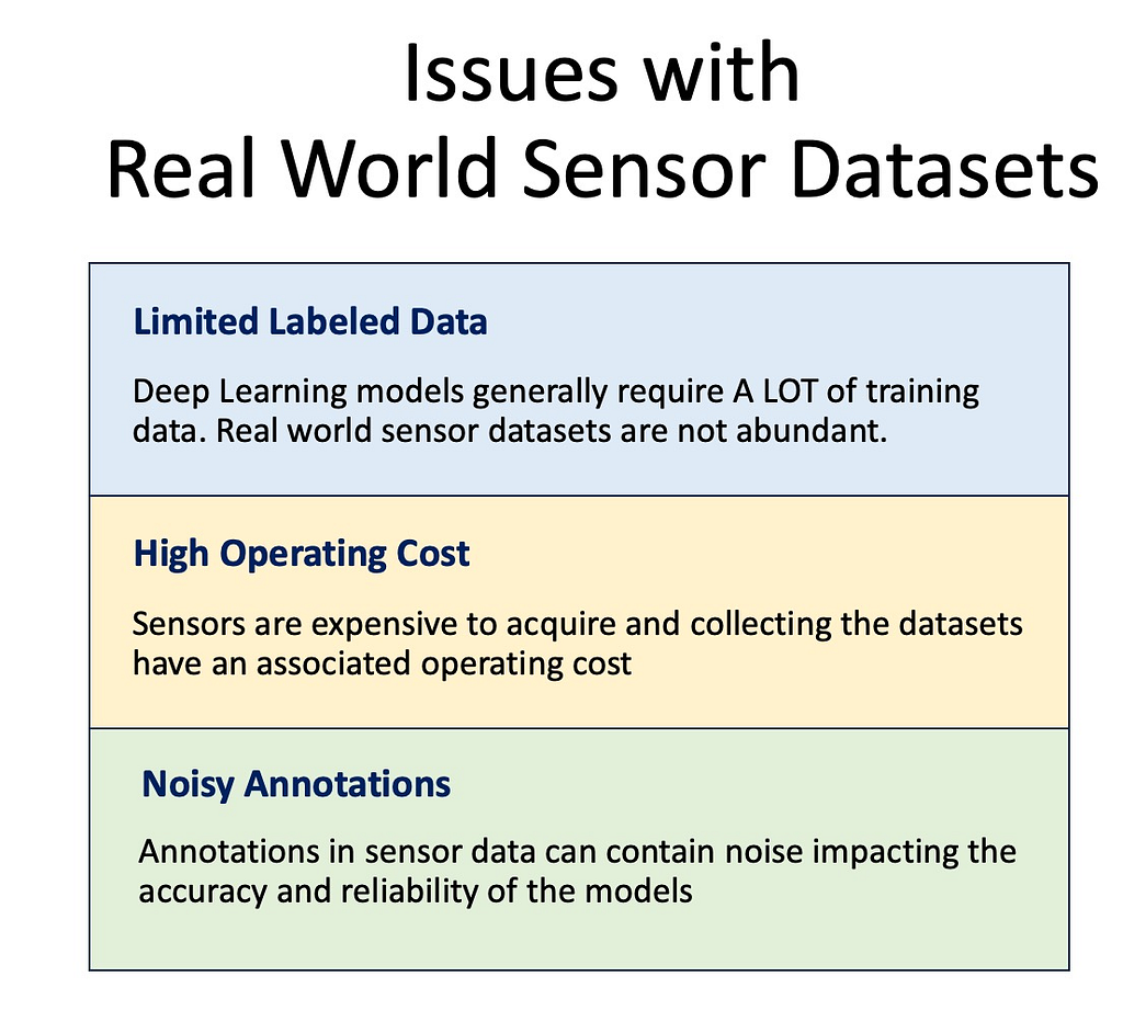
However, these methods come with several problems. The amount of labeled data is limited due to the high operational costs of obtaining these datasets. Additionally, the annotations can be noisy and low-resolution. Stereo cameras struggle under various lighting conditions and can’t reliably identify transparent or highly reflective surfaces. LiDAR is expensive, and both LiDAR and RGB-D cameras have limited range and generate low-resolution, sparse depth maps.

Can we use Unlabelled Images to learn Depth Estimation?

It would be beneficial to use unlabeled images to train depth estimation models, given the abundance of such images available online. The major innovation proposed in the original Depth Anything paper from 2023 was the incorporation of these unlabeled datasets into the training pipeline. In the next section, we’ll explore how this was achieved.

Depth Anything Architecture

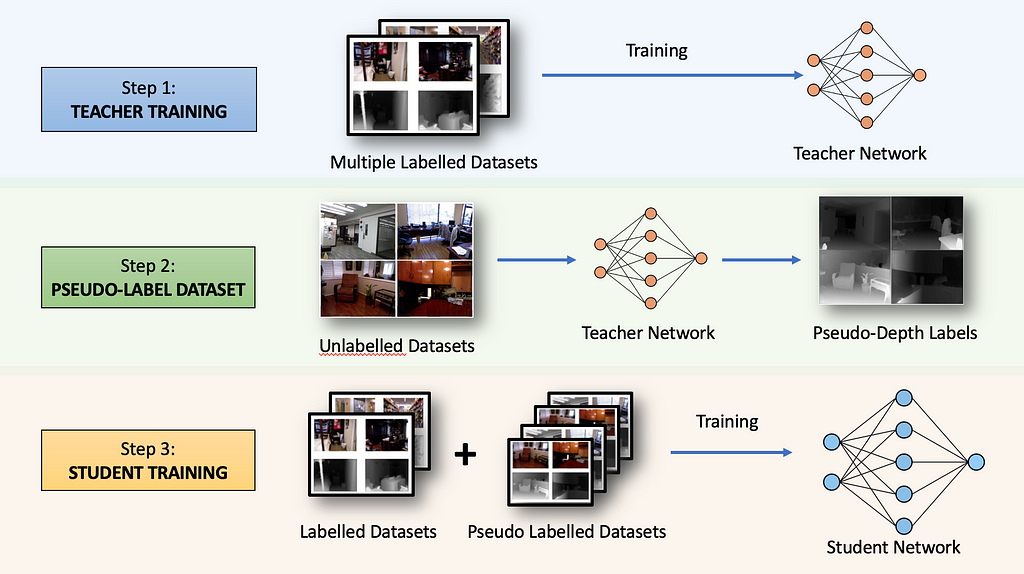
The original Depth Anything (V1) model from 2023 was trained in a three-step process. Let’s get a high-level overview of the algorithm before diving into each section.

Step 1: Teacher Training

First, a neural network called the TEACHER model is trained for supervised depth estimation using five different publicly available datasets.

Converting from Depth to Disparity Space

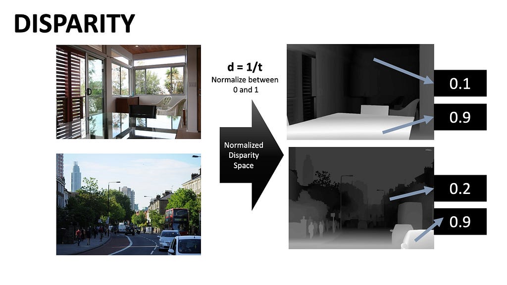
The TEACHER model is initialized with a pre-trained Dino-V2 encoder and then trained on the combined labeled dataset. A major challenge with training on multiple datasets is the variability in absolute depths. To address this, the depths are inverted into disparity space (d = 1 / t) and normalized between 0 and 1 for each depth map — 1 for the nearest pixel and 0 for the farthest. This way, all datasets share the same output space, allowing the model to predict disparity.

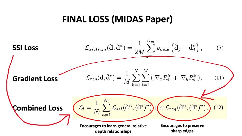
Two loss functions are used to train these models: a scale-shift invariant loss and a gradient-matching loss, both also utilized in the MiDAS paper from 2019.

1. Scale-shift invariant loss

There is a problem with using a simple mean square error loss between the predicted and ground truth images. Let’s say the ground truth depth values of three pixels in an image are 1, 0.5, and 0.1, while our network predicts 0.9, 0.6, and 0.3. Although the predictions aren’t exact, the relationship between the predicted and ground truth depths is similar, differing only by a multiplicative and additive factor. We don’t want this scale and shift to affect our loss function — we need to align the two maps before applying the mean square error loss.

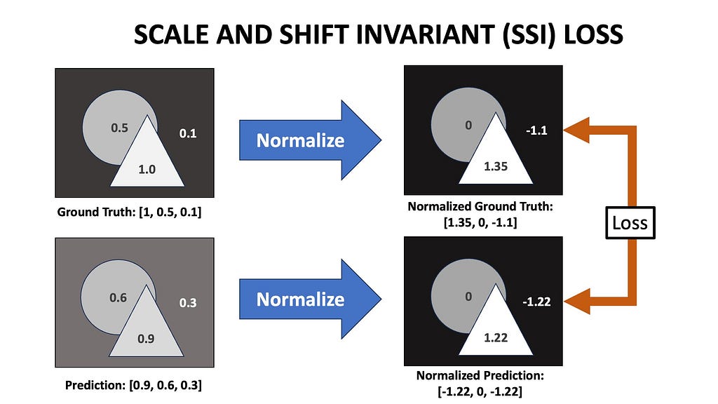
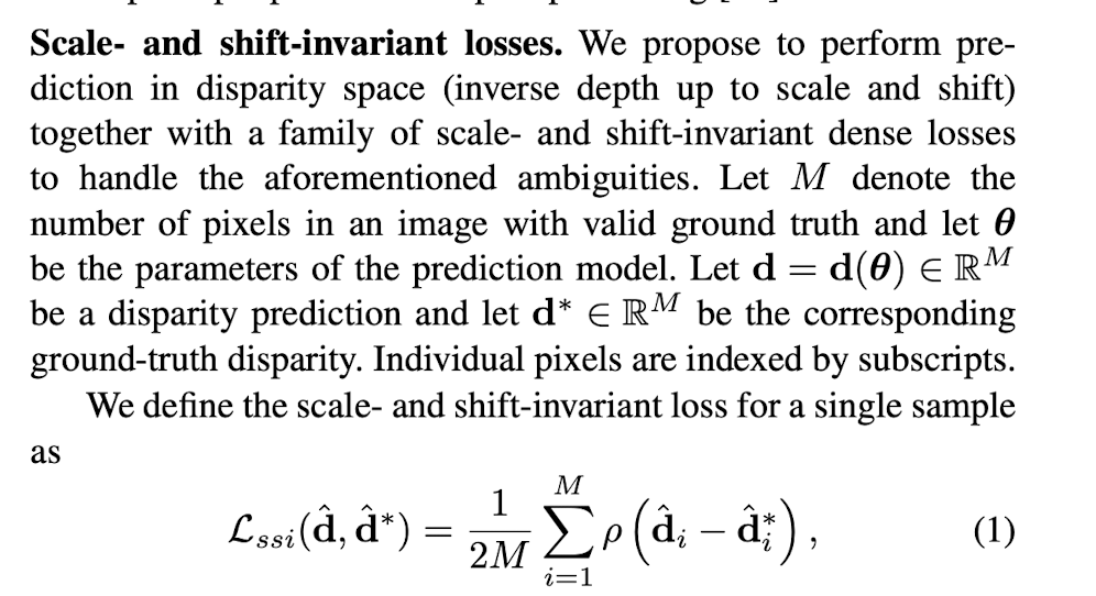
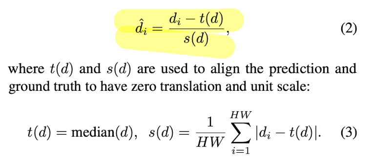
The MiDaS paper proposes normalizing the ground truth and predicted depths to have zero translation and unit scale. The median and deviation are calculated, and the depth maps are scaled and shifted accordingly. Once aligned, the mean square error loss is applied.

2. Gradient Matching Loss

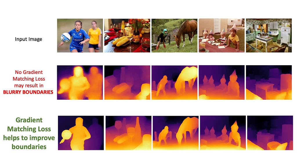
Using only the SSI loss might result in smoothed depth maps that fail to capture sharp distinctions between adjacent pixels. Gradient Matching Loss helps preserve these details by aligning the gradients of the predicted depth map with those of the ground truth.

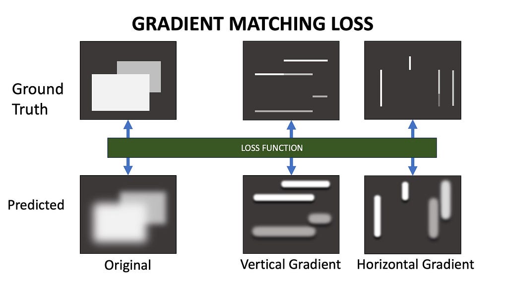
First, we calculate the gradients of the predicted and ground truth depth maps across the x and y axes, then apply the loss at the gradient level. MiDaS also uses a multi-scale gradient matching loss with four scale levels. The predicted and ground truth depth maps are downsampled four times, and the loss is applied at each resolution.

The final loss is the weighted sum of the scale-and-shift invariant loss and the multi-scale gradient matching loss. While the SSI loss encourages the model to learn general relative depth relationships, the gradient matching loss helps preserve sharp edges and fine-grained information in the scene.

Step 2 — Pseudo-Labelling Unlabelled Dataset

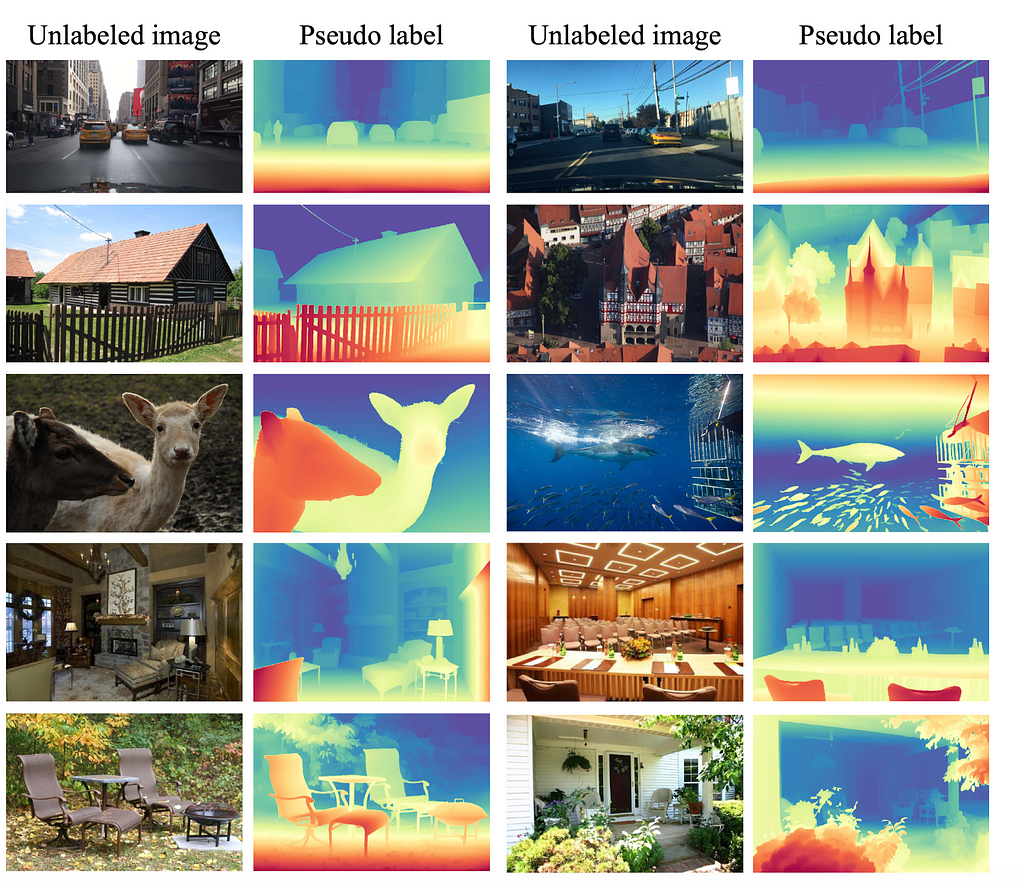
With our trained TEACHER model, we can now annotate millions of unlabeled images to create a massive pseudo-depth label dataset. These labels are called pseudo because they are AI-generated and may not represent the actual ground truth depth. We now have a lot of (pseudo) labeled images to train a new network.

Step 3 — Training Student Network

We will be training a new neural network (the student network) on the combination of the labeled and pseudo-labeled datasets. However, simply training the network on the annotations provided by the Teacher Network won’t improve the model beyond the capabilities of the base Teacher model. To make the student network more capable, two strategies were employed: heavy perturbations with image augmentations and introducing an auxiliary semantic preservation loss.

Heavy Perturbations

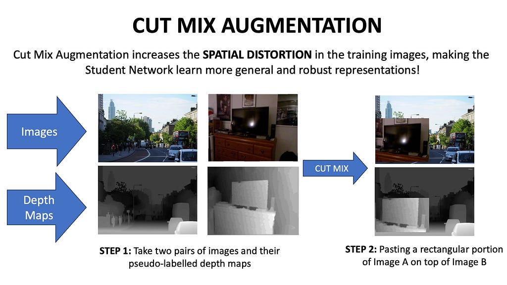
One interesting perturbation used was the Cut Mix operation. This involves combining a random pair of unlabeled images using a binary mask, replacing a rectangular portion of image A with image B. The final loss is the combined SSI and Gradient Matching loss of the two sections from the two ground truth depth maps. These spatial distortions are also combined with color distortions to help the Student Network handle the diversity of open-world images.

Auxiliary Semantic Preservation Loss

The network is also trained with an auxiliary task called Semantic Assisted Perception. A strong pre-trained computer vision model like Dino-V2, which has been trained on millions of images in a self-supervised manner, is used. Given an image, we aim to reduce the cosine distance between the embeddings produced by our new Student model and the pre-trained Dino-V2 encoder. This enables our Student model to capture some of the semantic perception capabilities of the larger and more general Dino-V2 model, which it uses to predict the depth map.

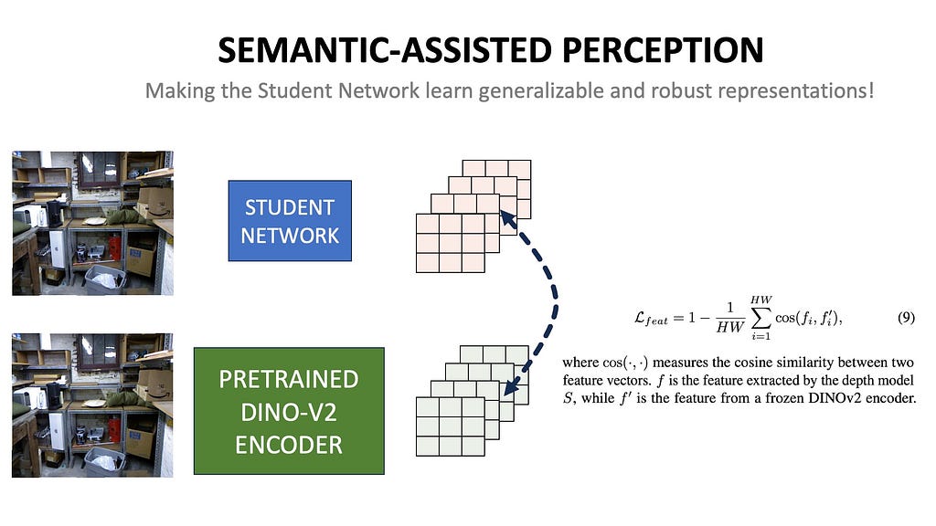
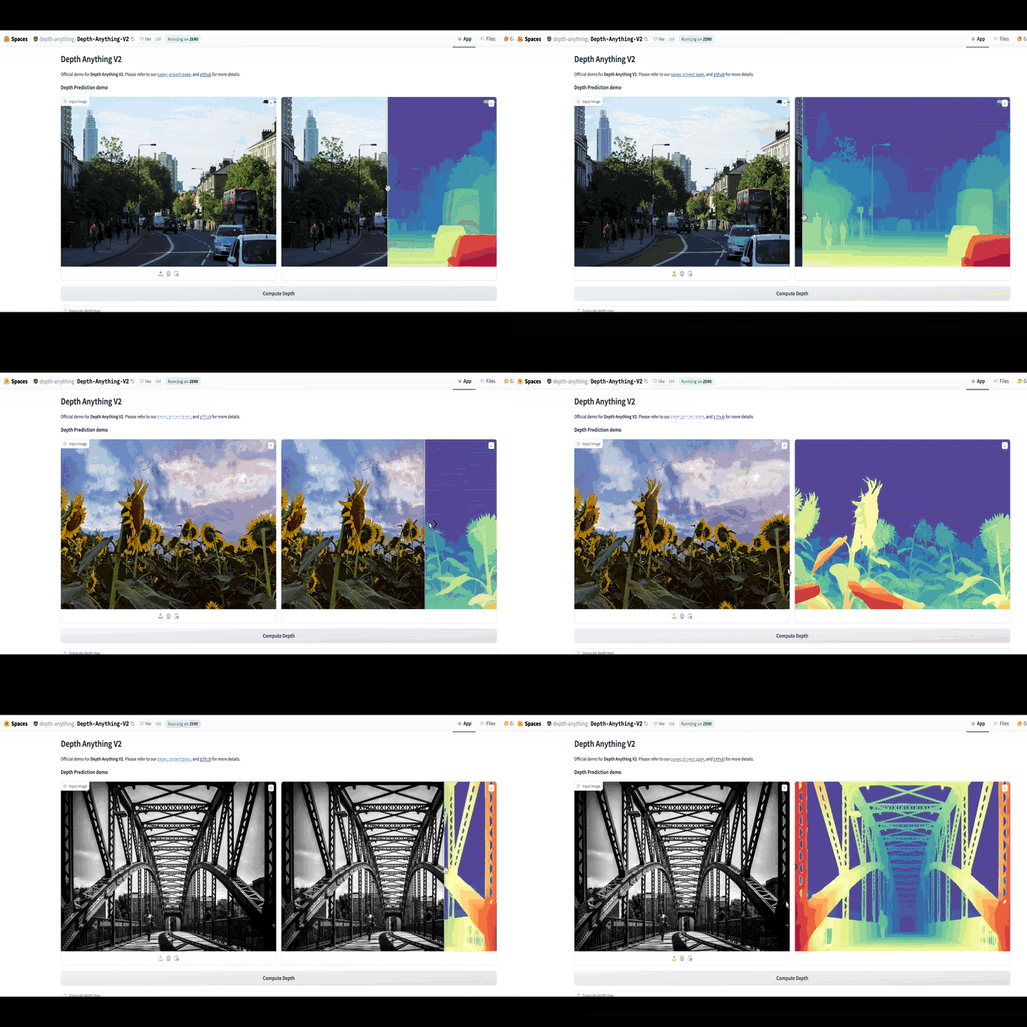
By combining spatial distortions, semantic-assisted perception, and the power of both labeled and unlabeled datasets, the Student Network generalizes better and outperforms the original Teacher Network in-depth estimation! Here are some incredible results from the Depth Anything V1 model!

Depth Anything V2

As impressive as Depth Anything V1’s results are, it struggles with transparent objects and capturing fine-grained details. The authors of Depth Anything V2 suggest that the biggest bottleneck for model performance isn’t the architecture itself, but the quality of the data. Most labeled datasets captured with sensors can be quite noisy, ignore fine-grained details, generate low-resolution depth maps, and struggle with lighting conditions and reflective/transparent objects.

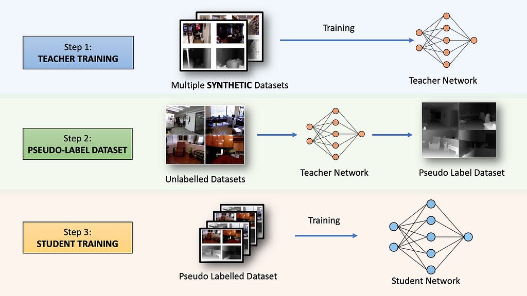
Depth Anything V2 discards labeled datasets from real-world sensors like stereo cameras, LiDAR, and RGB-D cameras, instead using only synthetic datasets. Synthetic datasets are generated through graphics engines, not captured with equipment. An example is the Virtual KITTI dataset, which uses the Unity Game Engine to create rendered images and depth maps for automated driving. There are also indoor datasets like IRS and Hyper-sim. Depth Anything V2 uses five synthetic datasets containing close to 595K photorealistic images.

Synthetic Datasets vs Real World Sensor Datasets

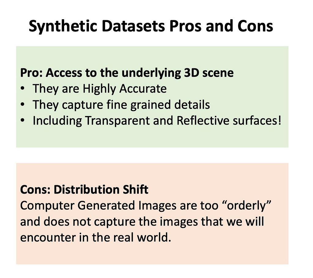
Synthetic images do have their pros and cons. They are super accurate, they have high-resolution outputs that capture the finest of the details, and the depth of transparent and reflective surfaces can be easily obtained. Synthetic datasets have direct access to all the 3D information needed since the graphics engine itself creates the scene.

On the cons side, these images may not essentially capture the images that we will encounter in real-world scenarios. The scene coverage of these datasets isn’t particularly diverse enough too, and is a much smaller subset of real-world images. Depth Anything 2 combines the power of synthetic images with millions of unlabelled images to train an MDE model that outperforms pretty much everything else we have seen so far.

Much like V1, the Teacher model in V2 is first trained on labeled datasets. However, in V2, it is exclusively trained on synthetic datasets. In Step 2, the Teacher model assigns pseudo-depth labels to all unlabeled images. Finally, in Step 3, the Student model is trained exclusively on pseudo-labeled images — no real labeled datasets and no synthetic datasets. The synthetic datasets are not used at this stage due to the distribution shift mentioned earlier. The Student network is trained on real-world images annotated by the Teacher model. Just like in V1, the auxiliary semantic preservation loss is used along with the Scale-and-Shift invariant and gradient matching loss.

Video link explaining the concepts here visually

Here is a video that explains all the concepts discussed in this video in a step-by-step method.

Depth Anything V1 vs Depth Anything V2

The original Depth Anything emphasized the importance of using unlabeled images in the MDE training pipeline. It introduced the knowledge distillation pipeline with Teacher training, pseudo-labeling unlabeled images, and then training the Student network on a combination of labeled and unlabeled images. The use of strong spatial and color distortions, and a semantic-assisted perception loss, helped create more general and robust embeddings. This resulted in efficient and high-quality depth maps for complex scenes. However, Depth Anything V1 still struggled with reflective surfaces and fine details due to noisy and low-resolution depth labels from real-world sensors.

Depth Anything V2 improved performance by ignoring real-world sensor datasets and only using synthetic images generated with graphics engines to train the Teacher Network. The Teacher Network then annotates millions of unlabeled images, and the Student Network is trained solely on these pseudo-labeled datasets with real-world images. With these techniques, Depth Anything V2 can now predict fine-level depth maps and handle transparent and reflective surfaces more effectively.

Relevant Links

MiDAS: https://arxiv.org/abs/1907.01341
Depth Anything: https://depth-anything.github.io/
Depth Anything V2: https://depth-anything-v2.github.io/

KITTI DATASET: https://www.cvlibs.net/datasets/kitti/
NYU V2: https://cs.nyu.edu/~fergus/datasets/nyu_depth_v2.html
VIRTUAL KITTI: https://datasetninja.com/virtual-kitti

Youtube Video: https://youtu.be/sz30TDttIBA

Monocular Depth Estimation with Depth Anything V2 was originally published in Towards Data Science on Medium, where people are continuing the conversation by highlighting and responding to this story.