Mastering Sample Size Calculations

A/B Testing, Reject Inference, and How to Get the Right Sample Size for Your Experiments

There are different statistical formulas for different scenarios. The first question to ask is: are you comparing two groups, such as in an A/B test, or are you selecting a sample from a population that is large enough to represent it?

The latter is typically used in cases like holdout groups in transactions. These holdout groups can be crucial for assessing the performance of fraud prevention rules or for reject inference, where machine learning models for fraud detection are retrained. The holdout group is beneficial because it contains transactions that weren’t blocked by any rules or models, providing an unbiased view of performance. However, to ensure the holdout group is representative, you need to select a sample size that accurately reflects the population, which, together with sample sizing for A/B testing, we’ll explore it in this article.

After determining whether you’re comparing two groups (like in A/B testing) or taking a representative sample (like for reject inference), the next step is to define your success metric. Is it a proportion or an absolute number? For example, comparing two proportions could involve conversion rates or default rates, where the number of default transactions is divided by the total number of transactions. On the other hand, comparing two means applies when dealing with absolute values, such as total revenue or GMV (Gross Merchandise Value). In this case, you would compare the average revenue per customer, assuming customer-level randomization in your experiment.

1. Comparing two groups (e.g. A/B testing) — Sample Size

The section 1.1 is about comparing two means, but most of the principles presented there will be the same for section 1.2.

1.1. Comparing two Means (metric the average of an absolute number)

In this scenario, we are comparing two groups: a control group and a treatment group. The control group consists of customers with access to €100 credit through a lending program, while the treatment group consists of customers with access to €200 credit under the same program.

The goal of the experiment is to determine whether increasing the credit limit leads to higher customer spending.

Our success metric is defined as the average amount spent per customer per week, measured in euros.

With the goal and success metric established, in a typical A/B test, we would also define the hypothesis, the randomization unit (in this case, the customer), and the target population (new customers granted credit). However, since the focus of this document is on sample size, we will not go into those details here.

We will compare the average weekly spending per customer between the control group and the treatment group. Let’s proceed with calculating this metric using the following script:

Script 1: Computing the success metric, branch: Germany, period: 2024–05–01 to 2024–07–31.

WITH customer_spending AS (
SELECT
 branch_id,
 FORMAT_DATE('%G-%V', DATE(transaction_timestamp)) AS week_of_year,
 customer_id,
 SUM(transaction_value) AS total_amount_spent_eur
FROM `project.dataset.credit_transactions`
WHERE 1=1
 AND transaction_date BETWEEN '2024-05-01' AND '2024-07-31'
 AND branch_id LIKE 'Germany'
GROUP BY branch_id, week_of_year, customer_id
)
, agg_per_week AS (
SELECT
 branch_id,
 week_of_year,
 ROUND(AVG(total_amount_spent_eur), 1) AS avg_amount_spent_eur_per_customer,
FROM customer_spending
GROUP BY branch_id, week_of_year
)
SELECT *
FROM agg_per_week
ORDER BY 1,2;

In the results, we observe the metric avg_amount_spent_eur_per_customer on a weekly basis. Over the last four weeks, the values have remained relatively stable, ranging between 35 and 54 euros. However, when considering all weeks over the past two months, the variance is higher. (See Image 1 for reference.)

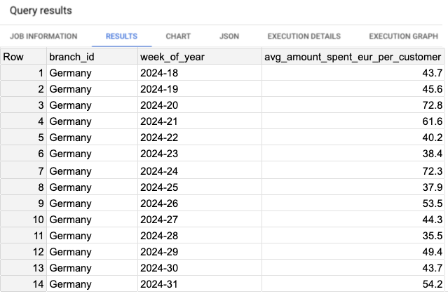
Next, we calculate the variance of the success metric. To do this, we will use Script 2 to compute both the variance and the average of the weekly spending across all weeks.

Script 2: Query to compute the variance of the success metric and average over all weeks.

WITH customer_spending AS (
SELECT
 branch_id,
 FORMAT_DATE('%G-%V', DATE(transaction_timestamp)) AS week_of_year,
 customer_id,
 SUM(transaction_value) AS total_amount_spent_eur
FROM `project.dataset.credit_transactions`
WHERE 1=1
 AND transaction_date BETWEEN '2024-05-01' AND '2024-07-31'
 AND branch_id LIKE 'Germany'
GROUP BY branch_id, week_of_year, customer_id
)
, agg_per_week AS (
SELECT
 branch_id,
 week_of_year,
 ROUND(AVG(total_amount_spent_eur), 1) AS avg_amount_spent_eur_per_customer,
FROM customer_spending
GROUP BY branch_id, week_of_year
)
SELECT
 ROUND(AVG(avg_amount_spent_eur_per_customer),1) AS avg_amount_spent_eur_per_customer_per_week,
 ROUND(VAR_POP(avg_amount_spent_eur_per_customer),1) AS variance_avg_amount_spent_eur_per_customer
FROM agg_per_week
ORDER BY 1,2;

The result from Script 2 shows that the variance is approximately 145.8 (see Image 2). Additionally, the average amount spent per user, considering all weeks over the past two months, is 49.5 euros.

Now that we’ve calculated the metric and found the average weekly spending per customer to be approximately 49.5 euros, we can define the Minimum Detectable Effect (MDE). Given the increase in credit from €100 to €200, we aim to detect a 10% increase in spending, which corresponds to a new average of 54.5 euros per customer per week.

With the variance calculated (145.8) and the MDE established, we can now plug these values into the formula to calculate the sample size required. We’ll use default values for alpha (5%) and beta (20%):

• Significance Level (Alpha’s default value is α = 5%): The alpha is a predetermined threshold used as a criteria to reject the null hypothesis. Alpha is the type I error (false positive), and the p-value needs to be lower than the alpha, so that we can reject the null hypothesis.
• Statistical Power (Beta’s default value is β = 20%): It’s the probability that a test correctly rejects the null hypothesis when the alternative hypothesis is true, i.e. detecting an effect when the effect is present. Statistical Power = 1 — β, and β is the type II error (false negative).

Here is the formula to calculate the required sample size per group (control and treatment) for comparing two means in a typical A/B test scenario:

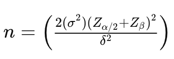
• n is the sample size per group.
• σ² is the variance of the metric being tested (in this case, 145.8). The factor 2σ² is used because we calculate the pooled variance, making it unbiased when comparing two samples.
• δ (Delta), represents the minimum detectable difference in means (effect size), which is the change we want to detect. That is calculated as: δ² = (μ₁ — μ₂)² , where μ₁ is the mean of the control group and μ₂ is the mean of the treatment group.
• Zα/2​ is the z-score for the corresponding confidence level (e.g., 1.96 for 95% confidence level).
• Zβ is the z-score associated with the desired power of the test (e.g., 0.84 for 80% power).

n = (2 * 145.8 * (1.96+0.84)^2) / (54.5-49.5)^2
-> n = 291.6 * 7.84 / 25
-> n = 2286.1 / 25
-> n =~ 92

Try it on my web app calculator at Sample Size Calculator, as shown in App Screenshot 1:

• Confidence Level: 95%
• Statistical Power: 80%
• Variance: 145.8
• Difference to Detect (Delta): 5 (because the expected change is from €49.50 to €54.50)

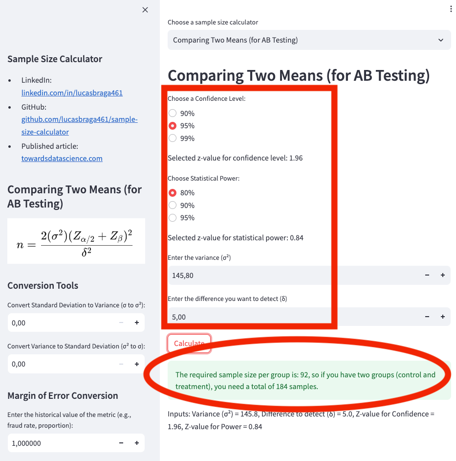
Based on the previous calculation, we would need 92 users in the control group and 92 users in the treatment group, for a total of 184 samples.

Now, let’s explore how changing the Minimum Detectable Effect (MDE) impacts the sample size. Smaller MDEs require larger sample sizes. For example, if we were aiming to detect a change of only €1 increase on average per user, instead of the €5 increase (10%) we used previously, the required sample size would increase significantly.

The smaller the MDE, the more sensitive the test needs to be, which means we need a larger sample to reliably detect such a small effect.

n = (2 * 145.8 * (1.96+0.84)^2) / (50.5-49.5)^2
-> n = 291.6 * 7.84 / 1
-> n = 2286.1 / 1
-> n =~ 2287

We enter the following parameters into the web app calculator at Sample Size Calculator, as shown in App Screenshot 2:

• Confidence Level: 95%
• Statistical Power: 80%
• Variance: 145.8
• Difference to Detect (Delta): 1 (because the expected change is from €49.50 to €50.50)

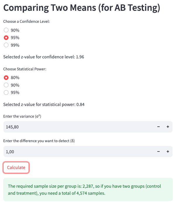
To detect a smaller effect, such as a €1 increase per user, we would require 2,287 users in the control group and 2,287 users in the treatment group, resulting in a total of 4,574 samples.

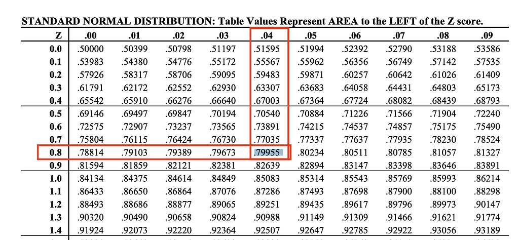
Next, we’ll adjust the statistical power and significance level to recompute the required sample size. But first, let’s take a look at the z-score table to understand how the Z-value is derived.

We’ve set beta = 0.2, meaning the current statistical power is 80%. Referring to the z-score table (see Image 4), this corresponds to a z-score of 0.84, which is the value used in our previous formula.

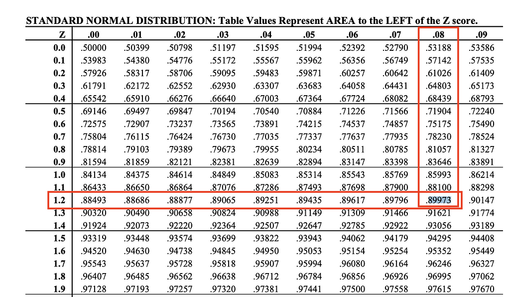
If we now adjust beta to 10%, which corresponds to a statistical power of 90%, we will find a z-value of 1.28. This value can be found on the z-score table (see Image 5).

n = (2 * 145.8 * (1.96+1.28)^2) / (50.5-49.5)^2
-> n = 291.6 * 10.49 / 1
-> n = 3061.1 / 1
-> n =~ 3062

With the adjustment to a beta of 10% (statistical power of 90%) and using the z-value of 1.28, we now require 3,062 users in both the control and treatment groups, for a total of 6,124 samples.

Now, let’s determine how much traffic the 6,124 samples represent. We can calculate this by finding the average volume of distinct customers per week. Script 3 will help us retrieve this information using the time period from 2024–05–01 to 2024–07–31.

Script 3: Query to calculate the average weekly volume of distinct customers.

WITH customer_volume AS (
SELECT
 branch_id,
 FORMAT_DATE('%G-%V', DATE(transaction_timestamp)) AS week_of_year,
 COUNT(DISTINCT customer_id) AS cntd_customers
FROM `project.dataset.credit_transactions`
WHERE 1=1
 AND transaction_date BETWEEN '2024-05-01' AND '2024-07-31'
 AND branch_id LIKE 'Germany'
GROUP BY branch_id, week_of_year
)
SELECT
 ROUND(AVG(cntd_customers),1) AS avg_cntd_customers
FROM customer_volume;

The result from Script 3 shows that, on average, there are 185,443 distinct customers every week (see Image 5). Therefore, the 6,124 samples represent approximately 3.35% of the total weekly customer base.

1.2. Comparing two Proportions (e.g. conversion rate, default rate)

While most of the principles discussed in the previous section remain the same, the formula for comparing two proportions differs. This is because, instead of pre-computing the variance of the metric, we will now focus on the expected proportions of success in each group (see Image 6).

Let’s return to the same scenario: we are comparing two groups. The control group consists of customers who have access to €100 credit on the credit lending program, while the treatment group consists of customers who have access to €200 credit in the same program.

This time, the success metric we are focusing on is the default rate. This could be part of the same experiment discussed in Section 1.1, where the default rate acts as a guardrail metric, or it could be an entirely separate experiment. In either case, the hypothesis is that giving customers more credit could lead to a higher default rate.

The goal of this experiment is to determine whether an increase in credit limits results in a higher default rate.

We define the success metric as the average default rate for all customers during the experiment week. Ideally, the experiment would run over a longer period to capture more data, but if that’s not possible, it’s essential to choose a week that is unbiased. You can verify this by analyzing the default rate over the past 12–16 weeks to identify any specific patterns related to certain weeks of the month.

Let’s examine the data. Script 4 will display the default rate per week, and the results can be seen in Image 7.

Script 4: Query to retrieve default rate per week.

SELECT
 branch_id,
 date_trunc(transaction_date, week) AS week_of_order,
 SUM(transaction_value) AS sum_disbursed_gmv,
 SUM(CASE WHEN is_completed THEN transaction_value ELSE 0 END) AS sum_collected_gmv,
 1-(SUM(CASE WHEN is_completed THEN transaction_value ELSE 0 END)/SUM(transaction_value)) AS default_rate,
FROM `project.dataset.credit_transactions`
WHERE transaction_date BETWEEN '2024-02-01' AND '2024-04-30'
  AND branch_id = 'Germany'
GROUP BY 1,2
ORDER BY 1,2;

Looking at the default rate metric, we notice some variability, particularly in the older weeks, but it has remained relatively stable over the past 5 weeks. The average default rate for the last 5 weeks is 0.070.

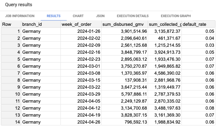
Now, let’s assume that this default rate will be representative of the control group. The next question is: what default rate in the treatment group would be considered unacceptable? We can set the threshold: if the default rate in the treatment group increases to 0.075, it would be too high. However, anything up to 0.0749 would still be acceptable.

A default rate of 0.075 represents approximately 7.2% increase from the control group rate of 0.070. This difference — 7.2% — is our Minimum Detectable Effect (MDE).

With these data points, we are now ready to compute the required sample size.

n = ( ((1.96+0.84)^2) * ((0.070*(1-0.070) + 0.075*(1-0.075)) ) / ( (0.070-0.075)^2 )
-> n = 7.84 * 0.134475 / 0.000025
-> n = 1.054284 / 0.000025
-> n =~ 42,171

We enter the following parameters into the web app calculator at Sample Size Calculator, as shown in App Screenshot 3:

• Confidence Level: 95%
• Statistical Power: 80%
• First Proportion (p1): 0.070
• Second Proportion (p2): 0.075

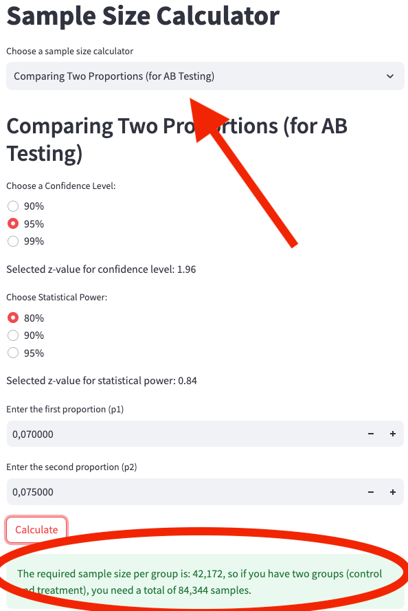
To detect a 7.2% increase in the default rate (from 0.070 to 0.075), we would need 42,171 users in both the control group and the treatment group, resulting in a total of 84,343 samples.

A sample size of 84,343 is quite large! We may not even have enough customers to run this analysis. But let’s explore why this is the case. We haven’t changed the default parameters for alpha and beta, meaning we kept the significance level at the default 5% and the statistical power at the default 80%. As we’ve discussed earlier, we could have been more conservative by choosing a lower significance level to reduce the chance of false positives, or we could have increased the statistical power to minimize the risk of false negatives.

So, what contributed to the large sample size? Is it the MDE of 7.2%? The short answer: not exactly.

Consider this alternative scenario: we maintain the same significance level (5%), statistical power (80%), and MDE (7.2%), but imagine that the default rate (p₁) was 0.23 (23%) instead of 0.070 (7.0%). With a 7.2% MDE, the new default rate for the treatment group (p₂) would be 0.2466 (24.66%). Notice that this is still a 7.2% MDE, but the proportions are significantly higher than 0.070 (7.0%) and 0.075 (7.5%).

Now, when we perform the sample size calculation using these new values of p₁ = 0.23 and p₂ = 0.2466, the results will differ. Let’s compute that next.

n = ( ((1.96+0.84)^2) * ((0.23*(1-0.23) + 0.2466*(1-0.2466)) ) / ( (0.2466-0.23)^2 )
-> n = 7.84 * 0.3628 / 0.00027556
-> n = 2.8450 / 0.00027556
-> n =~ 10,325

With the new default rates (p₁ = 0.23 and p₂ = 0.2466), we would need 10,325 users in both the control and treatment groups, resulting in a total of 20,649 samples. This is much more manageable compared to the previous sample size of 84,343. However, it’s important to note that the default rates in this scenario are in a completely different range.

The key takeaway is that lower success rates (like default rates around 7%) require larger sample sizes. When the proportions are smaller, detecting even modest differences (like a 7.2% increase) becomes more challenging, thus requiring more data to achieve the same statistical power and significance level.

2. Sampling a population

This case differs from the A/B testing scenario, as we are now focusing on determining a sample size from a single group. The goal is to take a sample that accurately represents the population, allowing us to run an analysis and then extrapolate the results to estimate what would happen across the entire population.

Even though we are not comparing two groups, sampling from a population (a single group) still requires deciding whether you are estimating a mean or a proportion. The formulas for these scenarios are quite similar to those used in A/B testing.

Take a look at images 8 and 9. Did you notice the similarities when comparing image 8 with image 3 (sample size formula for comparing two means) and when comparing image 9 with image 6 (sample size formula for comparing two proportions)? They are indeed quite similar.

In the case of estimating the mean:

• From image 8, the formula for sampling from one group, however, uses E, which stands for the Error.
• From image 3, the formula for comparing two groups uses delta (δ) to compare the difference between the two means.

In the case of estimating proportions:

• From image 9, for sampling from a single group, the formula for proportions also uses E instead, representing the Error.
• From image 6, the formula for comparing two groups uses the MDE (Minimum Detectable Effect), similar to delta, to compare the difference between two proportions.

Now, when should we use each of these formulas? Let’s explore two practical examples — one for estimating a mean and another for estimating a proportion.

2.1. Sampling a population — Estimating the mean

Let’s say you want to better assess the risk of fraud, and to do so, you aim to estimate the average order value of fraudulent transactions by country and per week. This can be quite challenging because, ideally, most fraudulent transactions are already being blocked. To get a clearer picture, you would take a holdout group that is free of rules and models, which would serve as a reference for calculating the true average order value of fraudulent transactions.

Suppose you select a specific country, and after reviewing historical data, you find that:

• The variance of this metric is €905.
• The average order value of fraudulent transactions is €100.
  (You can refer to Scripts 1 and 2 for calculating the success metric and variance.)

Since the variance is €905, the standard deviation (square root of variance) is approximately €30. Now, using a significance level of 5%, which corresponds to a z-score of 1.96, and assuming you’re comfortable with a 10% margin of error (representing an Error of €10, or 10% of €100), the confidence interval at 95% would mean that with the correct sample size, you can say with 95% confidence that the average value falls between €90 and €110.

Now, plugging these inputs into the sample size formula:

n = ( (1.96 * 30) / 10 )^2
-> n = (58.8/10)^2
-> n = 35

We enter the following parameters into the web app calculator at Sample Size Calculator, as shown in App Screenshot 4:

• Confidence Level: 95%
• Variance: 905
• Error: 10

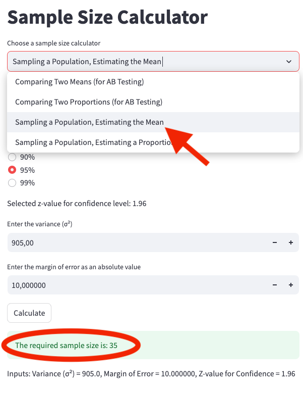
The result is that you would need 35 samples to estimate the average order value of fraudulent transactions per country per week. However, that’s not the final sample size.

Since fraudulent transactions are relatively rare, you need to adjust for the proportion of fraudulent transactions. If the proportion of fraudulent transactions is 1%, the actual number of samples you need to collect is:

n = 35/0.01
-> n = 3500

Thus, you would need 3,500 samples to ensure that fraudulent transactions are properly represented.

2.2. Sampling a population — Estimating a proportion

In this scenario, our fraud rules and models are blocking a significant number of transactions. To assess how well our rules and models perform, we need to let a portion of the traffic bypass the rules and models so that we can evaluate the actual false positive rate. This group of transactions that passes through without any filtering is known as a holdout group. This is a common practice in fraud data science teams because it allows for both evaluating rule and model performance and reusing the holdout group for reject inference.

Although we won’t go into detail about reject inference here, it’s worth briefly summarizing. Reject inference involves using the holdout group of unblocked transactions to learn patterns that help improve transaction blocking decisions. Several methods exist for this, with fuzzy augmentation being a popular one. The idea is to relabel previously rejected transactions using the holdout group’s data to train new models. This is particularly important in fraud modeling, where fraud rates are typically low (often less than 1%, and sometimes as low as 0.1% or lower). Increasing labeled data can improve model performance significantly.

Now that we understand the need to estimate a proportion, let’s dive into a practical use case to find out how many samples are needed.

For a certain branch, you analyze historical data and find that it processes 50,000,000 orders in a month, of which 50,000 are fraudulent, resulting in a 0.1% fraud rate. Using a significance level of 5% (alpha) and a margin of error of 25%, we aim to estimate the true fraud proportion within a confidence interval of 95%. This means if the true fraud rate is 0.001 (0.1%), we would be estimating a range between 0.00075 and 0.00125, with an Error of 0.00025.

Please note that margin of error and Error are two different things, the margin of error is a percentage value, and the Error is an absolute value. In the case where the fraud rate is 0.1% if we have a margin of error of 25% that represents an Error of 0.00025.

Let’s apply the formula:

• Zα/2 = 1.96 (z-score for 95% confidence level)
• E = 0.00025 (Error)
• p = 0.001 (fraud rate)

Zalpha/2= 1.96 
-> (Zalpha/2)^2= 3.8416
E = 0.00025
-> E^2 = 0.0000000625
p = 0.001

n =( 3.8416 * 0.001 * (1 - 0.001) ) / 0.0000000625
-> n = 0.0038377584 / 0.0000000625
-> n = 61,404

We enter the following parameters into the web app calculator at Sample Size Calculator, as shown in App Screenshot 5:

• Confidence Level: 95%
• Proportion: 0.001
• Error: 0.00025

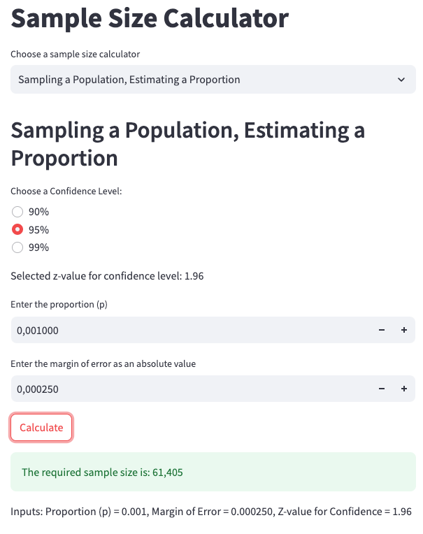
Thus, 61,404 samples are required in total. Given that there are 50,000,000 transactions in a month, it would take less than 1 hour to collect this many samples if the holdout group represented 100% of the traffic. However, this isn’t practical for a reliable experiment.

Instead, you would want to distribute the traffic across several days to avoid seasonality issues. Ideally, you would collect data over at least a week, ensuring representation from all weekdays while avoiding holidays or peak seasons. If you need to gather 61,404 samples in a week, you would aim for 8,772 samples per day. Since the daily traffic is around 1,666,666 orders, the holdout group would need to represent 0.53% of the total transactions each day, running over the course of a week.

Final notes

If you’d like to perform these calculations in Python, here are the relevant functions:

import math

def sample_size_comparing_two_means(variance, z_alpha, z_beta, delta):
   return math.ceil((2 * variance * (z_alpha + z_beta) ** 2) / (delta ** 2))

def sample_size_comparing_two_proportions(p1, p2, z_alpha, z_beta):
   numerator = (z_alpha + z_beta) ** 2 * ((p1 * (1 - p1)) + (p2 * (1 - p2)))
   denominator = (p1 - p2) ** 2
   return math.ceil(numerator / denominator)

def sample_size_estimating_mean(variance, z_alpha, margin_of_error):
   sigma = variance ** 0.5
   return math.ceil((z_alpha * sigma / margin_of_error) ** 2)

def sample_size_estimating_proportion(p, z_alpha, margin_of_error):
   return math.ceil((z_alpha ** 2 * p * (1 - p)) / (margin_of_error ** 2))

Here’s how you could calculate the sample size for comparing two means as in App screenshot 1 in section 1.1:

variance = 145.8
z_alpha = 1.96
z_beta = 0.84
delta = 5

sample_size_comparing_two_means(
    variance=variance, 
    z_alpha=z_alpha, 
    z_beta=z_beta, 
    delta=delta
)
# OUTPUT: 92

These functions are also available in the GitHub repository: GitHub Sample Size Calculator, this is also where you can find the link to the Interactive Sample Size Calculator.

Disclaimer: The images that resemble the results of a Google BigQuery job have been created by the author. The numbers shown are not based on any business data but were manually generated for illustrative purposes. The same applies to the SQL scripts — they are not from any businesses and were also manually generated. However, they are designed to closely resemble what a company using Google BigQuery as a framework might encounter.

• Calculator written in Python and deployed in Google Cloud Run (Serverless environment) using a Docker container and Streamlit, see code in GitHub for reference.

Mastering Sample Size Calculations was originally published in Towards Data Science on Medium, where people are continuing the conversation by highlighting and responding to this story.