Long-form video representation learning (Part 1: Video as graphs)

We explore novel video representations methods that are equipped with long-form reasoning capability. This is part 1 focusing on video representation as graphs and how to learn light-weights graph neural networks for several downstream applications. Part II focuses on sparse video-text transformers. And Part III provides a sneak peek into our latest and greatest explorations.

Existing video architectures tend to hit computation or memory bottlenecks after processing only a few seconds of the video content. So, how do we enable accurate and efficient long-form visual understanding? An important first step is to have a model that practically runs on long videos. To that end, we explore novel video representations methods that are equipped with long-form reasoning capability.

What is long-form reasoning and why ?

As we saw the huge leap of success of image-based understanding tasks with deep learning models such as convolutions or transformers, the next step naturally became going beyond still images and exploring video understanding. Developing video understanding models require two equally important focus areas. First is a large scale video dataset and the second is the learnable backbone for extracting video features efficiently. Creating finer-grained and consistent annotations for a dynamic signal such as a video is not trivial even with the best intention from both the system designer as well as the annotators. Naturally, the large video datasets that were created, took the relatively easier approach of annotating at the whole video level. About the second focus area, again it was natural to extend image-based models (such as CNN or transformers) for video understanding since videos are perceived as a collection of video frames each of which is identical in size and shape of an image. Researchers made their models that use sampled frames as inputs as opposed to all the video frames for obvious memory budget. To put things into perspective, when analyzing a 5-minute video clip at 30 frames/second, we need to process a bundle of 9,000 video frames. Neither CNN nor Transformers can operate on a sequence of 9,000 frames as a whole if it involves dense computations at the level of 16×16 rectangular patches extracted from each video frame. Thus most models operate in the following way. They take a short video clip as an input, do prediction, followed by temporal smoothing as opposed to the ideal scenario where we want the model to look at the video in its entirety.

Now comes this question. If we need to know whether a video is of type ‘swimming’ vs ‘tennis’, do we really need to analyze a minute-worth content? The answer is most certainly NO. In other words, the models optimized for video recognition, most likely learned to look at background and other spatial context information instead of learning to reason over what is actually happening in a ‘long’ video. We can term this phenomenon as learning the spatial shortcut. These models were good for video recognition tasks in general. Can you guess how do these models generalize for other tasks that require actual temporal reasoning such as action forecasting, video question-answering, and recently proposed episodic memory tasks? Since they weren’t trained for doing temporal reasoning, they turned out not quite good for those applications.

So we understand that datasets / annotations prevented most video models from learning to reason over time and sequence of actions. Gradually, researchers realized this problem and started coming up with different benchmarks addressing long-form reasoning. However, one problem still persisted which is mostly memory-bound i.e. how do we even make the first practical stride where a model can take a long-video as input as opposed to a sequence of short-clips processed one after another. To address that, we propose a novel video representation method based on Spatio-Temporal Graphs Learning (SPELL) to equip the model with long-form reasoning capability.

Video as a temporal graph

Let G = (V, E) be a graph with the node set V and edge set E. For domains such as social networks, citation networks, and molecular structure, the V and E are available to the system, and we say the graph is given as an input to the learnable models. Now, let’s consider the simplest possible case in a video where each of the video frame is considered a node leading to the formation of V. However, it is not clear whether and how node t1 (frame at time=t1) and node t2 (frame at time=t2) are connected. Thus, the set of edges, E, is not provided. Without E, the topology of the graph is not complete, resulting into unavailability of the “ground truth” graphs. One of the most important challenges remains how to convert a video to a graph. This graph can be considered as a latent graph since there is no such labeled (or “ground truth”) graph available in the dataset.

When a video is modeled as a temporal graph, many video understanding problems can be formulated as either node classification or graph classification problems. We utilize a SPELL framework for tasks such as Action Boundary Detection, Temporal Action Segmentation, Video summarization / highlight reels detection.

Video Summarization : Formulated as a node classification problem

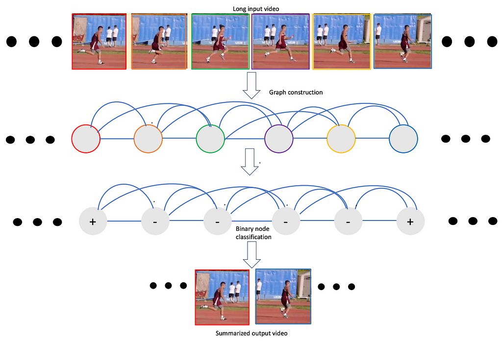
Here we present such a framework, namely VideoSAGE which stands for Video Summarization with Graph Representation Learning. We leverage the video as a temporal graph approach for video highlights reel creation using this framework. First, we convert an input video to a graph where nodes correspond to each of the video frames. Then, we impose sparsity on the graph by connecting only those pairs of nodes that are within a specified temporal distance. We then formulate the video summarization task as a binary node classification problem, precisely classifying video frames whether they should belong to the output summary video. A graph constructed this way (as shown in Figure 1) aims to capture long-range interactions among video frames, and the sparsity ensures the model trains without hitting the memory and compute bottleneck. Experiments on two datasets(SumMe and TVSum) demonstrate the effectiveness of the proposed nimble model compared to existing state-of-the-art summarization approaches while being one order of magnitude more efficient in compute time and memory.

We show that this structured sparsity leads to comparable or improved results on video summarization datasets(SumMe and TVSum) show that VideoSAGE has comparable performance as existing state-of-the-art summarization approaches while consuming significantly lower memory and compute budgets. The tables below show the comparative results of our method, namely VideoSAGE, on performances and objective scores. This has recently been accepted in a workshop at CVPR 2024. The paper details and more results are available here.

Action Segmentation : Formulated as a node classification problem

Similarly, we also pose the action segmentation problem as a node classification in such a sparse graph constructed from the input video. The GNN structure is similar to the above, except the last GNN layer is Graph Attention Network (GAT) instead of SageConv as used in the video summarization. We perform experiments of 50-Salads dataset. We leverage MSTCN or ASFormer as the stage 1 initial feature extractors. Next, we utilize our sparse, Bi-Directional GNN model that utilizes concurrent temporal “forward” and “backward” local message-passing operations. The GNN model further refine the final, fine-grain per-frame action prediction of our system. Refer to table 2 for the results.

Video as “object-centric” spatio-temporal graph

In this section, we will describe how we can take the similar graph based approach where as nodes denote “objects” instead of one whole video frame. We will start with a specific example to describe the spatio-temporal graph approach.

Active Speaker Detection : Task formulated as node classification

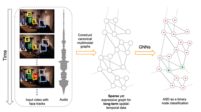
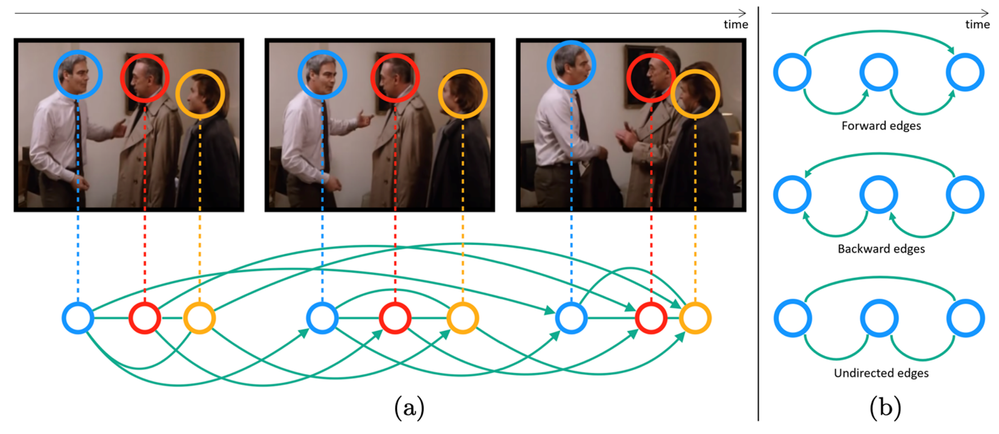
Figure 2 illustrates an overview of our framework designed for Active Speaker Detection (ASD) task. With the audio-visual data as input, we construct a multimodal graph and cast the ASD as a graph node classification task. Figure 3 demonstrates the graph construction process. First, we create a graph where the nodes correspond to each person within each frame, and the edges represent spatial or temporal relationships among them. The initial node features are constructed using simple and lightweight 2D convolutional neural networks (CNNs) instead of a complex 3D CNN or a transformer. Next, we perform binary node classification i.e. active or inactive speaker — on each node of this graph by learning a light-weight three-layer graph neural network (GNN). Graphs are constructed specifically for encoding the spatial and temporal dependencies among the different facial identities. Therefore, the GNN can leverage this graph structure and model the temporal continuity in speech as well as the long-term spatial-temporal context, while requiring low memory and computation.

You can ask why the graph construction is this way? Here comes the influence of the domain knowledge. The reason the nodes within a time distance that share the same face-id are connected with each other is to model the real-world scenario that if a person is taking at t=1 and the same person is talking at t=5, the chances are that person is talking at t=2,3,4. Why we connect different face-ids if they share the same time-stamp? That’s because, in general, if a person is talking others are most likely listening. If we had connected all nodes with each other and made the graph dense, the model not only would have required huge memory and compute, they would also have become noisy.

We perform extensive experiments on the AVA-ActiveSpeaker dataset. Our results show that SPELL outperforms all previous state-of-the-art (SOTA) approaches. Thanks to ~95% sparsity of the constructed graphs, SPELL requires significantly less hardware resources for the visual feature encoding (11.2M #Params) compared to ASDNet (48.6M #Params), one of the leading state-of-the-art methods of that time.

How long the temporal context is?

Refer to figure 3 below that shows the temporal context achieved by our methods on two different applications.

The hyper-parameter τ (= 0.9 second in our experiments) in SPELL imposes additional constraints on direct connectivity across temporally distant nodes. The face identities across consecutive timestamps are always connected. Below is the estimate of the effective temporal context size of SPELL. The AVA-ActiveSpeaker dataset contains 3.65 million frames and 5.3 million annotated faces, resulting in 1.45 faces per frame. Averaging 1.45 faces per frame, a graph with 500 to 2000 faces in sorted temporal order can span 345 to 1379 frames, corresponding to anywhere between 13 and 55 seconds for a 25 frame/second video. In other words, the nodes in the graph might have a time difference of about 1 minute, and SPELL is able to effectively reason over that long-term temporal window within a limited memory and compute budget. It is noteworthy that the temporal window size in MAAS is 1.9 seconds and TalkNet uses up to 4 seconds as long-term sequence-level temporal context.

The work on spatio-temporal graphs for active speaker detection has been published at ECCV 2022. The manuscript can be found here . In an earlier blog we provided more details.

Action Detection : Task formulated as node classification

The ASD problem setup in Ava active speaker dataset has access to the labeled faces and labeled face tracks as input to the problem setup. That largely simplifies the construction of the graph in terms of identifying the nodes and edges. For other problems, such as Action Detection, where the ground truth object (person) locations and tracks are not provided, we use pre-processing to detect objects and object tracks, then utilize SPELL for the node classification problem. Similar to the previous case, we utilize domain knowledge and contruct a sparse graph. The “object-centric” graphs are first created keeping the underlying application in mind.

On average, we achieve ~90% sparse graphs; a key difference compared to visual transformer-based methods which rely on dense General Matrix Multiply (GEMM) operations. Our sparse GNNs allow us to (1) achieve slightly better performance than transformer-based models; (2) aggregate temporal context over 10x longer windows compared to transformer-based models (100s vs 10s); and (3) Achieve 2–5X compute savings compared to transformers-based methods.

GraVi-T: Open Source Software Library

We have open-sourced our software library, GraVi-T. At present, GraVi-T supports multiple video understanding applications, including Active Speaker Detection, Action Detection, Temporal Segmentation, Video Summarization. See our opensource software library GraVi-T to more on the applications.

Highlights

Compared to transformers, our graph approach can aggregate context over 10x longer video, consumes ~10x lower memory and 5x lower FLOPs. Our first and major work in this topic (Active Speaker Detection) was published at ECCV’22. Watch out for our latest publication at upcoming CVPR 2024 on video summarization aka video highlights reels creation.

Our approach of modeling video as a sparse graph outperformed complex SOTA methods on several applications. It secured top places in multiple leaderboards. The list includes ActivityNet 2022, Ego4D audio-video diarization challenge at ECCV 2022, CVPR 2023. Source code for the training the past challenge winning models are also included in our open-sourced software library, GraVi-T.

We are excited about this generic, lightweight and efficient framework and are working towards other new applications. More exciting news coming soon !!!

Long-form video representation learning (Part 1: Video as graphs) was originally published in Towards Data Science on Medium, where people are continuing the conversation by highlighting and responding to this story.