Line-By-Line, Let’s Reproduce GPT-2: Section 2 — Hardware Optimization

Line-By-Line, Let’s Reproduce GPT-2: Section 2 — Hardware Optimization

This blog post will go line-by-line through the hardware optimizations in Section 2 of Andrej Karpathy’s “Let’s reproduce GPT-2 (124M)”

As a quick recap, in Section 1 we went line-by-line through the code written by Karpathy to naively train GPT-2. Now that we have our setup, Karpathy shows us how we can make the model train fast on our NVIDIA GPU! While we know that it takes a lot of time to train good models, by optimizing each run we can shave days or even weeks off our training time. This naturally gives us more iterations to improve our model. By the end of this blog post, you will see how to radically speed up your training (by 10x) using an Ampere-series Nvidia GPU.

To do this blog post, I ran the optimizations both on the NVIDIA T4 GPU that Google Colab gives you for free and on a NVIDIA A100 GPU 40GB SXM4 from Lambda Labs. Most of the optimizations Karpathy goes over are specifically for an A100 or better, but there are still some gains to be made on less powerful GPUs.

Let’s dive in!

Timing Our Code

To begin, we want to create a way to see how effective our optimizations are. To do so, we will add in to our training loop the below code:

for i in range(50):
    t0 = time.time() # start timer
    x, y = train_loader.next_batch()
    x, y = x.to(device), y.to(device)
    optimizer.zero_grad() 
    logits, loss = model(x, y)
    loss.backward() 
    optimizer.step()
    torch.cuda.synchronize() # synchronize with GPU
    t1 = time.time() # end timer
    dt = (t1-t0)*1000 # milliseconds difference
    print(f"loss {loss.item()}, step {i}, dt {dt:.2f}ms")

We start off by capturing the time at the beginning of the loop, but before we capture the end time we run torch.cuda.synchronize(). By default we are only paying attention to when the CPU stops. Because we have moved most of the major calculations to GPU, we need to make sure that our timer here takes into account when the GPU stops its calculations. Synchronize will have the CPU wait to progress until the GPU has completed its work queue, giving us an accurate time for when the loop was completed. Once we have an accurate time, we naturally calculate the difference between the start and the end.

Batch Sizing

We also want to make sure we are putting as much data as possible through each round. The way we achieve this is by setting batch sizes. In our DataLoaderLite class, we can adjust our 2 parameters (B and T) so that we use the most amount of memory in our GPU without going out of bounds.

With the A100 GPU, you can follow Karpathy’s example, where we set T equal to the max block_size of 1024 and we set B equal to 16 because it’s a “nice” number (easily divisible by powers of 2) and it’s the largest such “nice” number we can fit in memory.

train_loader = DataLoaderLite(B=16, T=1024)

If you try to put in a value that is too large, you’ll wind up seeing a OutOfMemoryError from CUDA in your terminal. I found the best values for a T4 GPU I could get was B =4 and T =1024 (when trying different B values in Google Colab, be aware you may need to restart the session to ensure you’re not getting false positive OutOfMemoryErrors)

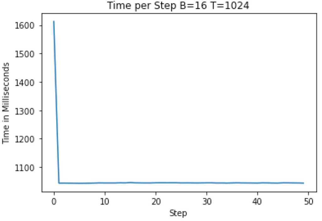
Running on the A100 and T4 below, I get the following graphs showing training time to start (on average roughly 1100ms on the T4 and 1040ms on the A100)

Floating Point Optimizations

Now we’re going to focus on changes we make to the internal representation of data within the model.

If you look at the dtype of the weights in our code from section 1, you will see we use Floating Point 32 (fp32) by default. Fp32 means that we represent the numbers using 32 bits following the IEEE floating point standard below:

As Karpathy says in the video, we have seen empirically that fp32 isn’t necessary to train quality models — we can use less data to represent each weight and still have quality outputs. One way to speed up the calculations is to use NVIDIA’s TensorCore instruction. This will handle the matrix multiplications by converting the operands to the form Tensor Float 32 (TF32) laid out below:

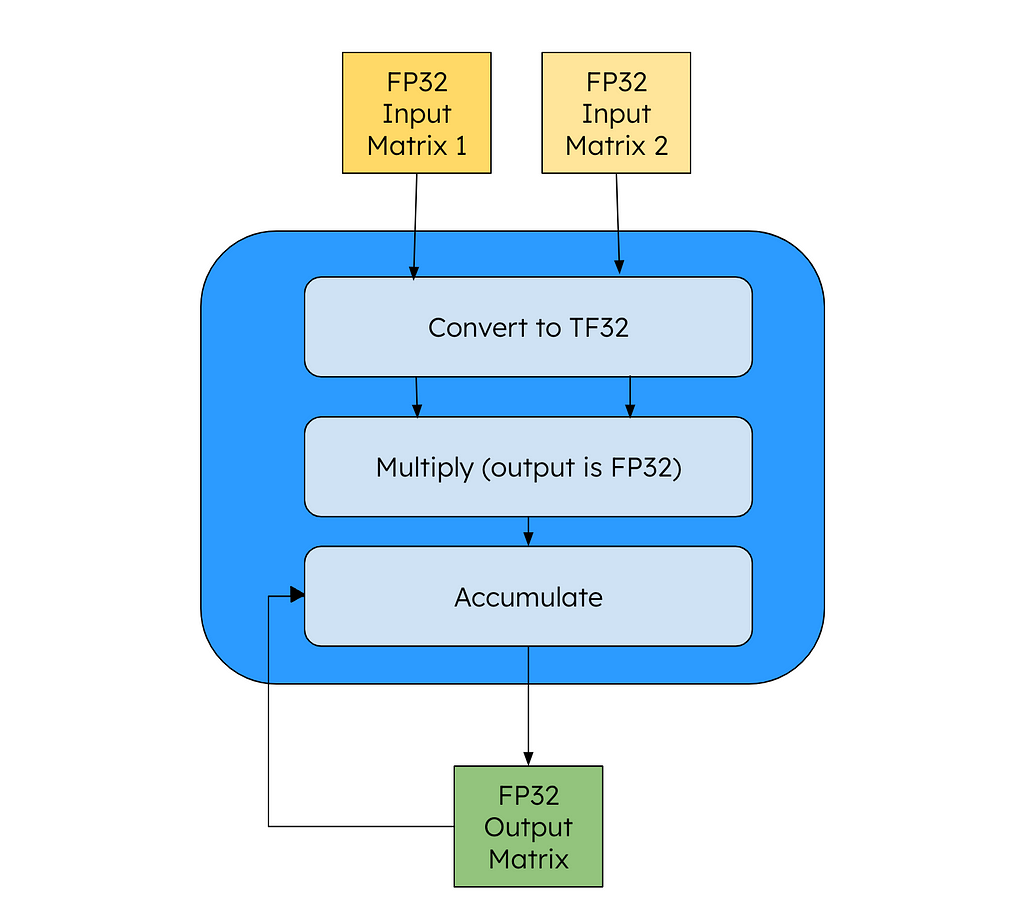
From the code point of view, all of our variables (input, output) are in FP32, but the NVIDIA GPU will convert the intermediary matrices to TF32 for speedup. This according to NVIDIA drives an 8x speed up versus a FFMA instruction. To enable TF32 in PyTorch, we only need to add the below line (high = TF32, highest = FP32, medium=BF16 (more on that later)):

torch.set_float32_matmul_precision("high")

TensorCore is unique to NVIDIA and you can only run TF32 on an A100 GPU or better, so some developers have used Floating Point 16 (FP16) as a way to train. The problem with this representation is that the range of data that FP16 can capture is smaller than FP32, leading to problems representing the same data range needed for training. While you can get around this using gradient expansion, this requires more calculations so you wind up in a situation where you take 1 step forwards, 2 steps back.

Instead, the data optimization Karpathy uses in his video is brain floating point (BF16). Here we have the same number of exponent bits as FP32, so we can represent the same range, but we have fewer mantissa bits. This means that while we have fewer bits, our precision in representing numbers is lower. Empirically, this has not caused major reduction in performance, so it’s a tradeoff we’re willing to make. To use this on NVIDIA chips, you need to have an A100.

Using PyTorch, we don’t need to change our code dramatically to use the new data type. The documentation advises us to only use these during the forward pass of your model and loss calculation. As our code does both of these in 1 line, we can modify our code as below:

for i in range(50):
    t0 = time.time() 
    x, y = train_loader.next_batch()
    x, y = x.to(device), y.to(device)
    optimizer.zero_grad() 
    with torch.autocast(device_type=device, dtype=torch.bfloat16): # bf16 change
        logits, loss = model(x, y)
    loss.backward() 
    optimizer.step()
    torch.cuda.synchronize() 
    t1 = time.time()
    dt = (t1-t0)*1000 
    print(f"loss {loss.item()}, step {i}, dt {dt:.2f}ms")
    loss_arr.append(loss.item())

Just like that, our code is now running using BF16.

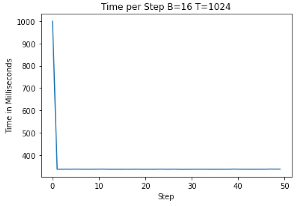
Running on our A100, we now see that the average step takes about 330ms! We’ve already reduced our runtime by about 70%, and we’re just getting started!

Torch Compile

We can further improve our training time by utilizing the PyTorch Compile feature. This will give us fairly big performance increases without having to adjust our code one bit.

To come at it from a high-level, every computer program is executed in binary. Because most people find it difficult to code in binary, we have created higher-level languages that let us code in forms that are easier for people to think in. When we compile these languages, they are transformed back into binary that we actually run. Sometimes in this translation, we can figure out faster ways to do the same calculation — such as reusing a certain variable or even simply not doing one to begin with.

# ...
model = GPT(GPTConfig(vocab_size=50304))
model.to(device)
model = torch.compile(model) # new line here
# ...

This brings us now to machine learning and PyTorch. Python is a high-level language but we’re still doing computationally intense calculations with it. When we run torch compile we are spending more time compiling our code, but we wind up seeing our runtime (the training for us here) go a lot faster because of that extra work we did to find those optimizations.

Karpathy gives the following example of how PyTorch may improve the calculations. Our GELU activation function can be written out like below:

class TanhGELU(nn.Module):
    def forward(self, input):
        return 0.5 * input * (1.0 + torch.tanh(math.sqrt(2.0/math.pi) * (input + 0.044715 * torch.pow(input, 3.0))))

For each calculation you see in the above function, we have to dispatch a kernel in the GPU. This means that when we start off by taking input to the third power, we pull input from high-bandwidth memory (HBM) into the GPU cores and do our calculation. We then write back to HBM before we start our next calculation and begin the whole process over again. Naturally, this sequencing is causing us to spend a lot of time waiting for memory transfers to occur.

PyTorch compile allows us to see an inefficiency like this and be more careful with when we are spinning up new kernels, resulting in dramatic speed ups. This is called kernel fusion.

While on this topic, I’d like to point out an excellent open-source project called Luminal that takes this idea a little further. Luminal is a separate framework that you write your training / inferencing in. By using this framework, you get access to its compiler which finds many more optimizations for you by nature of having a more limited number of computations to consider. If you like the idea of improving runtime by compiling fast GPU code, give the project a look.

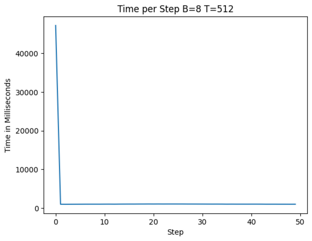
When we run the above code now we see that we see each step takes roughly 145 ms (cutting by 50% from before and ~86% from the original). We pay for this with the first iteration which took roughly 40,000ms to run! As most training sequences have many more steps than 50, this tradeoff is one that we are willing to make.

Flash Attention

Another optimization we make is using Flash Attention (see the paper here). The code change itself is very simple for us, but the thinking behind it is worth exploring.

y = F.scaled_dot_product_attention(q, k, v, is_causal=True)

Similar to how we condensed the TanhGELU class into as few kernels as we could, we apply the same thinking to attention. In their paper, “FlashAttention: Fast and Memory-Efficient Exact Attention with IO-Awareness”, the authors show how you can achieve a 7.6x speed up by fusing the kernel. While in theory torch compile should be able to find optimizations like this, in practice we haven’t seen it find this yet.

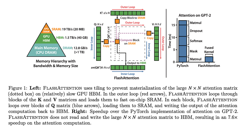
The paper is worth doing a deep dive on, but to give a quick synopsis, FlashAttention is written to be IO-aware, thus preventing unnecessary (and time-consuming) calls to memory. By reducing these, they can radically speed up the calculations.

After implementing this, we find that we now have an average step of about 104ms.

Vocab Size Change

Finally, we can go through all of the numbers we have hard-coded and evaluate how “nice” they are. When we do this, we find that the vocabulary size is not divisible by many powers of 2 and so will be more time-consuming for our GPU’s memory to load in. We fix this by going from the 50,257 vocab size to the next “nice” number, which is 50,304. This is a nice number as it’s cleanly divisible by 2, 4, 8, 16, 32, 64, and 128.

model = GPT(GPTConfig(vocab_size=50304))

Now you may remember from the last blog post that our vocab size is not an arbitrary value — it is determined by the tokenizer we are using. Thus begs the question, When we arbitrarily add in more values to our vocab size, what happens? During the training, the model will notice that these new vocab never appear, so it will start to push the probabilities of these tokens to 0 — thus our performance is safe. That does not mean that there is no tradeoff though. By loading into memory vocab that is never used, we are wasting time. However, empirically we can see that loading in “nice” numbers more than compensates for this cost.

With our last optimization, we now have an average of about 100 ms per step.

With this final optimization, we find that our training has improved ~10x from the beginning!

What optimizations work on T4 GPU?

If you’ve been following along but only have access to the consumer-grade T4 GPU, you may wonder which optimizations you can use. To recap, we cannot use the BF16 representation, but we can use the vocabulary size change, flash attention, and torch compile. To see this code in action, check out my Google Colab notebook, which is optimized just for T4 usage.

We can see from the graph below that while the torch compile does take a lot of time for the first round, the next rounds are not significantly better than the unoptimized versions (roughly an 8% drop on T4 vs 90% drop on A100).

Nevertheless, when OpenAI was training GPT-2 it was running on far more advanced hardware than the T4. The fact that we can run this workload on a T4 today suggests that hardware requirements are becoming less onerous, helping create a future where hardware is not a barrier to ML work.

Closing

By optimizing our code, we’ve seen major speed ups and also learned a bit about where the big bottlenecks for training happen. First and foremost, datatypes are critically important for speed, as this change by itself contributed majorly to the speed ups. Second, we see that hardware optimizations can play a major role in speeding up calculations — so GPU hardware is worth its weight in gold. Finally, compiler optimizations have a major role to play here as well.

To see the code I ran in the A100, check out this gist here. If you have any suggestions for how to optimize the hardware further, I would love to see them in the comments!

It’s an exciting time to be building!

[1] Karpathy, A., “Let’s reproduce GPT-2 (124M)” (2024), YouTube

[2] Dao, T., et al. “FlashAttention: Fast and Memory-Efficient Exact Attention with IO-Awareness” (2022), arXiv

[3] Krashinsky, R., et al “NVIDIA Ampere Architecture In-Depth” (2020), NVIDIA Developer

Line-By-Line, Let’s Reproduce GPT-2: Section 2 — Hardware Optimization was originally published in Towards Data Science on Medium, where people are continuing the conversation by highlighting and responding to this story.