Let’s reproduce NanoGPT with JAX!(Part 1)

Part 1: Build 124M GPT2 with JAX.
Part 2: Optimize the training speed in Single GPU.
Part 3: Multi-GPU Training in Jax.

Inspired by Andrej Kapathy’s recent youtube video on Let’s reproduce GPT-2 (124M), I’d like to rebuild it with most of the training optimizations in Jax. Jax is built for highly efficient computation speed, and it is quite interesting to compare Pytorch with its recent training optimization, and Jax with its related libraries like Flax (Layers API for neural network training for Jax)and Optax (a gradient processing and optimization library for JAX). We will quickly learn what is Jax, and rebuild the GPT with Jax. In the end, we will compare the token/sec with multiGPU training between Pytorch and Jax!

What is Jax?

Based on its readthedoc, JAX is a Python library for accelerator-oriented array computation and program transformation, designed for high-performance numerical computing and large-scale machine learning. I would like to introduce JAX with its name. While someone calls it Just Another XLA (Accelerated Linear Algibra), I prefer to call it J(it) A(utograd) X(LA) to demonstrate its capability of high efficiency.

J — Just-in-time (JIT) Compilation. When you run your python function, Jax converts it into a primitive set of operation called Jaxpr. Then the Jaxpr expression will be converted into an input for XLA, which compiles the lower-level scripts to produce an optimized exutable for target device (CPU, GPU or TPU).

A — Autograd. Computing gradients is a critical part of modern machine learning methods, and you can just call jax.grad() to get gradients which enables you to optimize the models.

X — XLA. This is a open-source machine learning compiler for CPU, GPU and ML accelerators. In general, XLA performs several built-in optimization and analysis passes on the StableHLO graph, then sends the HLO computation to a backend for further HLO-level optimizations. The backend then performs target-specific code generation.

Those are just some key features of JAX, but it also has many user friendly numpy-like APIs in jax.numpy , and automatic vectorization with jax.vmap , and parallize your codes into multiple devices via jax.pmap . We will cover more Jax concepts nd applications in the futher blogs, but now let’s reproduct the NanoGPT with Jax!

From Attention to Transformer

GPT is a decoder-only transformer model, and the key building block is Attention module. We can first define a model config dataclass to save the model hyperparameters of the model, so that the model module can consume it efficiently to initialize the model architecture. Similar to the 124M GPT model, here we initialize a 12-layer transformer decoder with 12 heads and vocab size as 50257 tokens, each of which has 768 embedding dimension. The block size for the attention calculation is 1024.

from dataclasses import dataclass

@dataclass
class ModelConfig:
  vocab_size: int = 50257
  n_head: int = 12
  n_embd: int = 768
  block_size: int = 1024
  n_layer: int = 12
  dropout_rate: float = 0.1

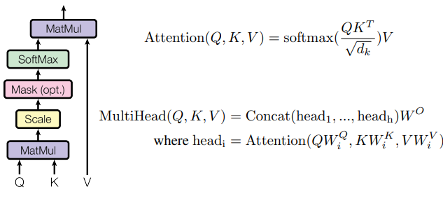
Next comes to the key building block of the transformer model — Attention. The idea is to process the inputs into three weight matrics: Key, Query, and Value. Here we rely on the flax , a the Jax Layer and training API library to initialize the 3 weight matrix, by just call the flax.linen.Dense . As mentioned, Jax has many numpy-like APIs, so we reshape the outputs after the weight matrix with jax.numpy.reshape from [batch_size, sequence_length, embedding_dim] to [batch_size, sequence_length, num_head, embedding_dim / num_head]. Since we need to do matrix multiplication on the key and value matrics, jax also has jax.numpy.matmul API and jax.numpy.transpose (transpose the key matrix for multiplication).

Note that we need to put a mask on the attention matrix to avoid information leakage (prevent the previous tokens to have access to the later tokens), jax.numpy.tril helps build a lower triangle array, and jax.numpy.where can fill the infinite number for us to get 0 after softmax jax.nn.softmax . The full codes of multihead attention can be found below.

from flax import linen as nn
import jax.numpy as jnp

class CausalSelfAttention(nn.Module):

  config: ModelConfig

  @nn.compact
  def __call__(self, x, deterministic=True):

    assert len(x.shape) == 3

    b, l, d = x.shape

    q     = nn.Dense(self.config.n_embd)(x)
    k     = nn.Dense(self.config.n_embd)(x)
    v     = nn.Dense(self.config.n_embd)(x)
    # q*k / sqrt(dim) -> softmax -> @v
    q     = jnp.reshape(q, (b, l, d//self.config.n_head , self.config.n_head))
    k     = jnp.reshape(k, (b, l, d//self.config.n_head , self.config.n_head))
    v     = jnp.reshape(v, (b, l, d//self.config.n_head , self.config.n_head))
    norm  = jnp.sqrt(list(jnp.shape(k))[-1])
    attn  = jnp.matmul(q,jnp.transpose(k, (0,1,3,2))) / norm
    mask  = jnp.tril(attn)
    attn  = jnp.where(mask[:,:,:l,:l], attn, float("-inf"))
    probs = jax.nn.softmax(attn, axis=-1)
    y     = jnp.matmul(probs, v)
    y     = jnp.reshape(y, (b,l,d))
    y     = nn.Dense(self.config.n_embd)(y)
    return y

You may notice that there is no __init__ or forward methods as you can see in the pytorch. This is the special thing for jax, where you can explicitly define the layers with setup methods, or implicitly define them withn the forward pass by adding nn.compact on top of __call__ method. [ref]

Next let’s build the MLP and Block layer, which includes Dense layer, Gelu activation function, LayerNorm and Dropout. Again flax.linen has the layer APIs to help us build the module. Note that we will pass a deterministic boolean variable to control different behaviors during training or evaluation for some layers like Dropout.

class MLP(nn.Module):

  config: ModelConfig

  @nn.compact
  def __call__(self, x, deterministic=True):
    x = nn.Dense(self.config.n_embd*4)(x)
    x = nn.gelu(x, approximate=True)
    x = nn.Dropout(rate=self.config.dropout_rate)(x, deterministic=deterministic)
    x = nn.Dense(self.config.n_embd)(x)
    x = nn.Dropout(rate=self.config.dropout_rate)(x, deterministic=deterministic)
    return x

class Block(nn.Module):

  config: ModelConfig

  @nn.compact
  def __call__(self, x):
    x = nn.LayerNorm()(x)
    x = x + CausalSelfAttention(self.config)(x)
    x = nn.LayerNorm()(x)
    x = x + MLP(self.config)(x)
    return x

Now Let’s use the above blocks to build the NanoGPT:

Given the inputs of a sequence token ids, we use the flax.linen.Embed layer to get position embeddings and token embeddings. Them we pass them into the Block module N times, where N is number of the layers defined in the Model Config. In the end, we map the outputs from the last Block into the probabilities for each token in the vocab to predict the next token. Besides the forward __call__ method, let’s also create a init methods to get the dummy inputs to get the model’s parameters.

class GPT(nn.Module):

  config: ModelConfig

  @nn.compact
  def __call__(self, x, deterministic=False):
    
    B, T = x.shape
    assert T <= self.config.block_size

    pos     = jnp.arange(0, T)[None]
    pos_emb = nn.Embed(self.config.block_size, self.config.n_embd)(pos)
    wte     = nn.Embed(self.config.vocab_size, self.config.n_embd)
    tok_emb = wte(x)
    x       = tok_emb + pos_emb

    for _ in range(self.config.n_layer):
      x = Block(self.config)(x)
    x = nn.LayerNorm()(x)
    logits = nn.Dense(config.n_embd, config.vocab_size)
    # logits = wte.attend(x) # parameter sharing
    return logits
  
  def init(self, rng):
    tokens = jnp.zeros((1, self.config.block_size), dtype=jnp.uint16)
    params = jax.jit(super().init, static_argnums=(2,))(rng, tokens, True)
    return params

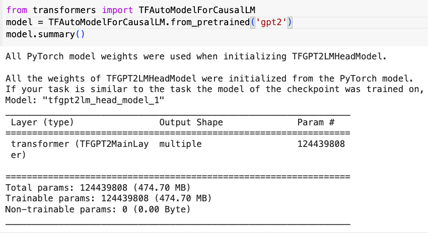
Now let’s varify the number of parameters: We first initialize the model config dataclass and the random key, then create a dummy inputs and feed in into the GPT model. Then we utilize the jax.util.treemap API to create a count parameter function. We got 124439808 (124M) parameters, same amount as Huggingface’s GPT2, BOOM!

DataLoader and Training Loop

Let’s now overfit a small dataset. To make it comparable inAndrej’s video on Pytorch NanoGPT, let’s use the toy dataset that he shared in his video. We use the GPT2′ tokenizer from tiktoken library to tokenize all the texts from the input file, and convert the tokens into jax.numpy.array for Jax’s model training.

class DataLoader:
  def __init__(self, B, T):
    self.current_position = 0
    self.B = B
    self.T = T

    with open("input.txt","r") as f:
      text = f.read()
    enc = tiktoken.get_encoding("gpt2")
    self.tokens = jnp.array(enc.encode(text))
    print(f"loaded {len(self.tokens)} tokens in the datasets" )
    print(f" 1 epoch = {len(self.tokens)//(B*T)} batches")

  def next_batch(self):
    B,T = self.B, self.T
    buf = self.tokens[self.current_position:self.current_position+B*T+1]
    x,y = jnp.reshape(buf[:-1],(B,T)), jnp.reshape(buf[1:],(B,T))
    self.current_position += B*T
    if self.current_position + B*T+1 > len(self.tokens):
      self.current_position = 0
    return x,y

Next, let’s forget distributed training and optimization first, and just create a naive training loop for a sanity check. The first thing after intialize the model is to create a TrainState, a model state where we can update the parameters and gradients. The TrainState takes three important inputs: apply_fn (model forward function), params (model parameters from the init method), and tx (an Optax gradient transformation).

Then we use the train_step function to update the model state (gradients and parameters) to proceed the model training. Optax provide the softmax cross entropy as the loss function for the next token prediction task, and jax.value_and_grad calculates the gradients and the loss value for the loss function. Finally, we update the model’s state with the new parameters using the apply_gradients API. [ref] Don’t forget to jit the train_step function to reduce the computation overhead!

def init_train_state(key, config) -> TrainState:
  model = GPT(config)
  params = model.init(key)
  optimizer = optax.adamw(3e-4, b1=0.9, b2=0.98, eps=1e-9, weight_decay=1e-1)
  train_state = TrainState.create(
        apply_fn=model.apply,
        params=params,
        tx=optimizer)
  return train_state

@jax.jit
def train_step(state: TrainState, x: jnp.ndarray, y: jnp.ndarray) -> Tuple[jnp.ndarray, TrainState]:

  def loss_fn(params: FrozenDict) -> jnp.ndarray:

      logits = state.apply_fn(params, x, False)
      loss = optax.softmax_cross_entropy_with_integer_labels(logits, y).mean()
      return loss

  loss, grads = jax.value_and_grad(loss_fn, has_aux=False)(state.params)
  new_state = state.apply_gradients(grads=grads)
  return loss, new_state

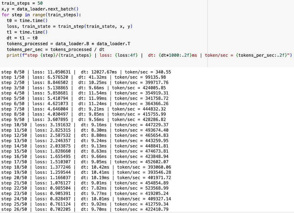
Now everything is ready for the poorman’s training loop.. Let’s check the loss value. The model’s prediction should be better than the random guess, so the loss should be lower than -ln(1/50257)≈10.825. What we expect from the overfitting a single batch is that: in the beginning the loss is close to 10.825, then it goes down to close to 0. Let’s take a batch of (x, y) and run the training loop for 50 times. I also add similar log to calculate the training speed.

As we can see, the loss value is exactly what we expect, and the training throughput is around 400–500 k token/sec. Which is already 40x faster than Pytorch’s initial version without any optimization in Andrej’s video. Note that we run the Jax scripts in 1 A100 GPU which should remove the hardware difference for the speed comparison. There is no .to(device) stuff to move your model or data from host CPU to device GPU, which is one of the benefits from Jax!

So that’s it and we made it. We will make the training 10x more faster in Part 2 with more optimizations…

Part 2: The journey of training optimization to 1350k tokens/sec in a single GPU!

“Unless otherwise noted, all images are by the author”

Let’s reproduce NanoGPT with JAX!(Part 1) was originally published in Towards Data Science on Medium, where people are continuing the conversation by highlighting and responding to this story.