Jointly learning rewards and policies: an iterative Inverse Reinforcement Learning framework with ranked synthetic trajectories
A novel tractable and interpretable algorithm to learn from expert demonstrations

Introduction
Imitation Learning has recently gained increasing attention in the Machine Learning community, as it enables the transfer of expert knowledge to autonomous agents through observed behaviors. A first category of algorithm is Behavioral Cloning (BC), which aims to directly replicate expert demonstrations, treating the imitation process as a supervised learning task where the agent attempts to match the expert’s actions in given states. While straightforward and computationally efficient, BC often suffers from overfitting and poor generalization.
In contrast, Inverse Reinforcement Learning (IRL) targets the underlying intent of expert behavior by inferring a reward function that could explain the expert’s actions as optimal within the considered environment. Yet, an important caveat of IRL is the inherent ill-posed nature of the problem — i.e. that multiple (if not possibly an infinite number of) reward functions can make the expert trajectories as optimal. A widely adopted class of methods to tackle this ambiguity includes Maximum Entropy IRL algorithms, which introduce an entropy maximization term to encourage stochasticity and robustness in the inferred policy.
In this article, we choose a different route and introduce a novel iterative IRL algorithm that jointly learns both the reward function and the optimal policy from expert demonstrations alone. By iteratively synthesizing trajectories and guaranteeing their increasing quality, our approach departs from traditional IRL models to provide a fully tractable, interpretable and efficient solution.
The organization of the article is as follows: section 1 introduces some basic concepts in IRL. Section 2 gives an overview of recent advances in the IRL literature, which our model builds on. We derive a sufficient condition for the our model to converge in section 3. This theoretical result is general and can apply to a large class of algorithms. In section 4, we formally introduce the full model, before concluding on key differences with existing literature and further research directions in section 5.
1. Background definitions:
First let’s define a few concepts, starting with the general Inverse Reinforcement Learning problem (note: we assume the same notations as this article):
An Inverse Reinforcement Learning (IRL) problem is a 5-tuple (S, A, P, γ, τ*) such that:
- S is the set of states the agent can be in
- A is the set of actions the agent can take
- P are transition probabilities
- γ ∈ (0, 1] is a discount factor
- τ* is the set of expert demonstrations, i.e. τ*ᵢ = (sᵢ, aᵢ) is a sequence of actions (sometimes called trajectory) taken by an expert agent
The goal of Inverse Reinforcement Learning is to infer the reward function R of the MDP (S, A, R, P, γ) solely from the expert trajectories. The expert is assumed to have full knowledge of this reward function and acts in a way that maximizes the reward of his actions.
We make the additional assumption of linearity of the reward function (common in IRL literature) i.e. that it is of the form:

where ϕ is a static feature map of the state-action space and w a weight vector. In practice, this feature map can be found via classical Machine Learning methods (e.g. VAE — see [6] for an example). The feature map can therefore be estimated separately, which reduces the IRL problem to inferring the weight vector w rather than the full reward function.
In this context, we finally derive the feature expectation μ, which will prove useful in the different methods presented. Starting from the value function of a given policy π:

We then use the linearity assumption of the reward function introduced above:
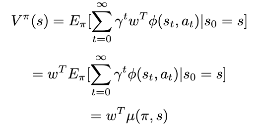
Likewise, μ can also be computed separately — usually via Monte Carlo.
2. Related work in RL and IRL literature
2.1 Apprenticeship Learning:
A seminal method to learn from expert demonstrations is Apprenticeship learning, first introduced in [1]. Unlike pure Inverse Reinforcement Learning, the objective here is to both to find the optimal reward vector as well as inferring the expert policy from the given demonstrations. We start with the following observation:

Mathematically this can be seen using the Cauchy-Schwarz inequality. This result is actually quite powerful, as it allows to focus on matching the feature expectations, which will guarantee the matching of the value functions — regardless of the reward weight vector.
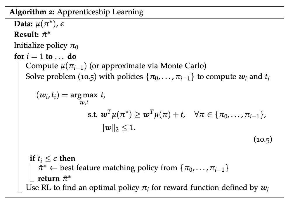
In practice, Apprenticeship Learning uses an iterative algorithm based on the maximum margin principle to approximate μ(π*) — where π* is the (unknown) expert policy. To do so, we proceed as follows:
- Start with a (potentially random) initial policy and compute its feature expectation, as well as the estimated feature expectation of the expert policy from the demonstrations (estimated via Monte Carlo)
- For the given feature expectations, find the weight vector that maximizes the margin between μ(π*) and the other (μ(π)). In other words, we want the weight vector that would discriminate as much as possible between the expert policy and the trained ones
- Once this weight vector w’ found, use classical Reinforcement Learning — with the reward function approximated with the feature map ϕ and w’ — to find the next trained policy
- Repeat the previous 2 steps until the smallest margin between μ(π*) and the one for any given policy μ(π) is below a certain threshold — meaning that among all the trained policies, we have found one that matches the expert feature expectation up to a certain ϵ
Written more formally:
2.2 IRL with ranked demonstrations:
The maximum margin principle in Apprenticeship Learning does not make any assumption on the relationship between the different trajectories: the algorithm stops as soon as any set of trajectories achieves a narrow enough margin. Yet, suboptimality of the demonstrations is a well-known caveat in Inverse Reinforcement Learning, and in particular the variance in demonstration quality. An additional information we can exploit is the ranking of the demonstrations — and consequently ranking of feature expectations.
More precisely, consider ranks {1, …, k} (from worst to best) and feature expectations μ₁, …, μₖ. Feature expectation μᵢ is computed from trajectories of rank i. We want our reward function to efficiently discriminate between demonstrations of different quality, i.e.:

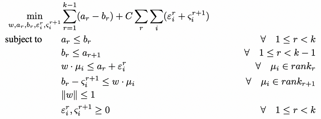
In this context, [5] presents a tractable formulation of this problem into a Quadratic Program (QP), using once again the maximum margin principle, i.e. maximizing the smallest margin between two different classes. Formally:

This is actually very similar to the optimization run by SVM models for multiclass classification. The all-in optimization model is the following — see [5] for details:
2.3 Disturbance-based Reward Extrapolation (D-REX):
Presented in [4], the D-REX algorithm also uses this concept of IRL with ranked preferences but on generated demonstrations. The intuition is as follows:
- Starting from the expert demonstrations, imitate them via Behavioral cloning, thus getting a baseline π₀
- Generate ranked sets of demonstration with different degrees of performance by injecting different noise levels to π₀: in [4] authors prove that for two levels of noise ϵ and γ, such that ϵ > γ (i.e. ϵ is “noisier” than γ) we have with high probability that V[π(. | ϵ)] < V[π’. | γ)]- where π(. | x) is the policy resulting from injecting noise x in π₀.
- Given this automated ranking provided, run an IRL from ranked demonstrations method (T-REX) based on approximating the reward function with a neural network trained with a pairwise loss — see [3] for more details
- With the approximation of the reward function R’ gotten from the IRL step, run a classical RL method with R’ to get the final policy
More formally:

Another important theoretical result presented in [4] is the effect of ranking on reward ambiguity: the paper manages to quantify the ambiguity reduction coming from added ranking constraint, which elegantly tackles the ill-posed nature of IRL.
2.4 Guided Reinforcement Learning:
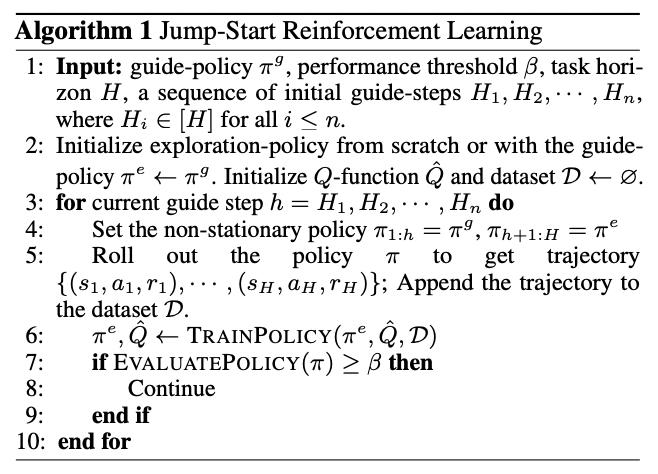
How can we leverage some expert demonstrations when fitting a Reinforcement Learning model? Rather than start exploring using an initial random policy, one could think of leveraging available demonstration information — as suboptimal as they might be — as a warm start and guide at least the beginning of the RL training. This idea is formalized in [8], and the intuition is:
- For each training iteration, start with the expert policy / demonstrations (πᵍ) — to collect “good” samples and put the agent in “good” states
- After a determined switch point, let the current trained policy (πᵉ) take over and explore states — the objective being that it explores states that have not been visited (enough) by the expert demonstrations, while relying on the expert choices for the visited ones
- As it gets better, πᵉ should take over earlier
More formally:
3. A sufficient condition for convergence:
Before deriving the full model, we establish the following result that will provide a useful bound guaranteeing improvement in an iterative algorithm — full proof is provided in the Appendix:
Theorem 1: Let (S, A, P, γ, π*) the Inverse Reinforcement Learning problem with unknown true reward function R*. For two policies π₁ and π₂ fitted using the candidate reward functions R₁ and R₂ of the form Rᵢ = R* + ϵᵢ with ϵᵢ some error function, we have the following sufficient condition to have π₂ improve upon π₁, i.e. V(π₂, R*) > V(π₁, R*):

Where TV(π₂, π₁) is the total variation distance between π₂ and π₁, interpreting the policies as probability measures.
This bound gives some intuitive insights, since if we want to guarantee improvement on a known policy with its reward function, the margin gets higher the more:
- Different the two reward functions are
- Different the two policies are
- Imprecise the original reward function is
4. The full tractable model
Building on the previously introduced models and Theorem 1, we can derive our new fully tractable model. The intuition is:
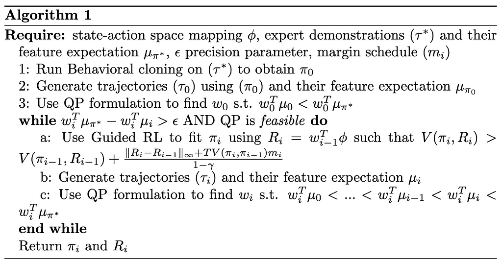
- Initialization: start from the expert trajectories (τ*), estimate an initial policy π₀ (e.g. via Behavioral Cloning) and generate trajectories (τ₀) of an agent following π₀. Use these trajectories to estimate a reward weight vector w₀ (which gives R₀ = w₀ ϕ )such that V(π*, R₀) > V(π₀, R₀) through the Quadratic Program presented in section 2.2 — i.e. the ranking here being: {2 : τ*, 1: τ₀}
- Iteration: infer a policy πᵢ using wᵢ-₁ (i.e. Rᵢ = wᵢ-₁ϕ) such that we have V(πᵢ, Rᵢ) > V(πᵢ-₁, Rᵢ-₁) with sufficient margin using Guided RL. Note that here we do not necessarily want πᵢ to be optimal w.r.t. Rᵢ, we simply want something that outperforms the current policy by a certain margin as dictated by Theorem 1. The rationale behind this is that we do not want to overfit on the inaccuracies caused by the reward misspecification. See [7] for more details on the impact of this misspecification.
- Likewise, generate samples τᵢ with policy πᵢ and use the tractable IRL model on the following updated ranking: {i : τ*, i-1: τᵢ, i-2: τᵢ-₁…}
- Stopping condition: when V(τ*, wᵢ) — V(τᵢ, wᵢ) is below a certain threshold ϵ or if the Quadratic Program is infeasible
Formally:
This algorithm makes a few choices that we need to keep in mind:
- An implicit assumption we make is that the reward functions are getting more precise through the iterations, i.e. the noise terms ϵᵢ are decreasing in norm and go to 0
- Since the noise terms ϵᵢ are unknown, we replace them with a predetermined margin schedule (mᵢ)— following the above assumption we can make the schedule decreasing and going to 0
- Why stop the iteration if the QP is infeasible: we know that the QP was feasible at the previous iteration, therefore the main constraint that made it infeasible was adding the new feature expectation μᵢ computed with trajectories using πᵢ. We interpret this infeasibility as the fact that we’re unable to get a margin significant enough to discriminate between μᵢ and μ*, which can mean that wᵢ-₁ and πᵢ are optimal solutions.
5. Conclusion and future work:
While synthesizing multiple models from RL and IRL literature, this new heuristic innovates in a number of ways:
- Full tractability: not using a neural network for the IRL step is a choice, as it enhances tractability and interpretability. It also provides additional insights related to the feasibility of the QP which can allow to stop the algorithm earlier.
- Efficiency and ease of use: although an iterative algorithm, each step of the iteration can be done very efficiently: the QP can be solved quickly using current solvers and the RL step requires only a limited number of iterations to satisfy the improvement condition presented in Theorem 1. It also offers additional flexibility with the ϵ coefficient, allowing the user to “pay” some suboptimality for faster convergence if needed.
- Better use of all information available to minimize noise: the iterative nature of the algorithm limits the uncertainty propagation from IRL to RL as we always restart the fitting (offering a possibility to course-correct). The Guided RL step also allows to introduce a healthy bias towards the expert demonstrations.
We can also note that Theorem 1 is a general property and provides a bound that can be applied to a large class of algorithms.
Further research can naturally be done to extend this algorithm. First, a thorough implementation and benchmarking against other approaches can provide interesting insights. Another direction would be deepening the theoretical study of the convergence conditions of the model, especially the assumption of reduction of reward noise.
Appendix:
We prove Theorem 1 introduced earlier similarly to the proof of Theorem 1 in [4]. The target inequality for two given policies fitted at steps i and i-1 is: V(πᵢ, R*) > V(πᵢ-₁, R*). The objective is to derive a sufficient condition for this inequality to hold. We start with the following assumptions:
- π₁ is the policy fitted at the previous iteration using the reward function R₁
- The RL step uses a form of iterative algorithm (e.g. Value Iteration), which yields that at the current iteration π₂ is also known — even if it is only a candidate policy that could be improved if it does not fit the condition. The reward function it is (currently being) fitted on is R₂
- The reward functions Rᵢ are of the form: Rᵢ = R* + ϵᵢ with ϵᵢ some error function
We thus have:
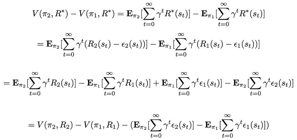
Following the assumptions mades, V(π₂, R₂) — V(π₁, R₁) is known at the time of the iteration. For the second part of the expression featuring ϵ₁ and ϵ₂ (which are unknown, as we only know ϵ₁ — ϵ₂ = R₁ — R₂) we derive an upper bound for its value:
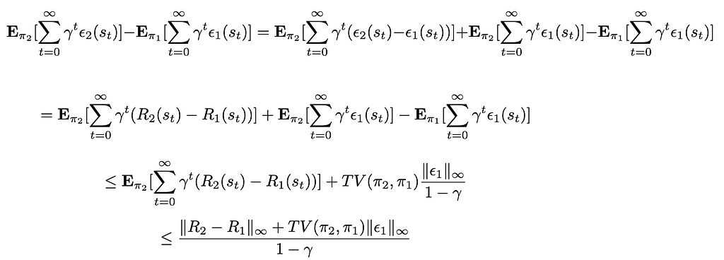
Where TV(π₁, π₂) is the total variance between π₁ and π₂, as we interpret the policies as probability measures. We reinject this upper bound in the first expression, giving:

Therefore, this gives the following condition to have the policy π₂ improve on π₁:

References:
[1] P. Abbeel, A. Y. Ng, Apprenticeship Learning via Inverse Reinforcement Learning (2004), Stanford Artificial Intelligence Laboratory
[2] J. Bohg, M. Pavone, D. Sadigh, Principles of Robot Autonomy II (2024), Stanford ASL web
[3] D. S. Brown, W. Goo, P. Nagarajan, S. Niekum, Extrapolating Beyond Suboptimal Demonstrations via Inverse Reinforcement Learning from Observations (2019), Proceedings of Machine Learning Research
[4] D. S. Brown, W. Goo, P. Nagarajan, S. Niekum, Better-than-Demonstrator Imitation Learning via Automatically-Ranked Demonstrations (2020), Proceedings of Machine Learning Research
[5] P. S. Castro, S. Li, D. Zhang, Inverse Reinforcement Learning with Multiple Ranked Experts (2019), arXiv
[6] A. Mandyam, D. Li, D. Cai, A. Jones, B. E. Engelhardt, Kernel Density Bayesian Inverse Reinforcement Learning (2024), arXiv
[7] A. Pan, K. Bhatia, J. Steinhardt, The Effects of Reward Misspecification: Mapping and Mitigating Misaligned Models (2022), arXiv
[8] I. Uchendu, T. Xiao, Y. Lu, B. Zhu, M. Yan, J. Simon, M. Bennice, Ch. Fu, C. Ma, J. Jiao, S. Levine, K. Hausman, Jump-Start Reinforcement Learning (2023), Proceedings of Machine Learning Research
Jointly learning rewards and policies: an iterative Inverse Reinforcement Learning framework with… was originally published in Towards Data Science on Medium, where people are continuing the conversation by highlighting and responding to this story.
Originally appeared here:
Jointly learning rewards and policies: an iterative Inverse Reinforcement Learning framework with…