Is Multi-Collinearity Destroying Your Causal Inferences In Marketing Mix Modelling?

Causal AI, exploring the integration of causal reasoning into machine learning

What is this series about?

Welcome to my series on Causal AI, where we will explore the integration of causal reasoning into machine learning models. Expect to explore a number of practical applications across different business contexts.

In the last article we covered powering experiments with CUPED and double machine learning. Today, we shift our focus to understanding how multi-collinearity can damage the causal inferences you make, particularly in marketing mix modelling.

If you missed the last article on powering experiments with CUPED and double machine learning, check it out here:

Powering Experiments with CUPED and Double Machine Learning

Introduction

In this article, we will explore how damaging multi-collinearity can be and evaluate some methods we can use to address it. The following aspects will be covered:

• What is multi-collinearity?
• Why is it a problem in causal inference?
• Why is it so common in marketing mix modelling?
• How can we detect it?
• How can we address it?
• An introduction to Bayesian priors.
• A Python case study exploring how Bayesian priors and random budget adjustments can help alleviate multi-collinearity.

The full notebook can be found here:

causal_ai/notebooks/is multi-collinearity destroying your mmm.ipynb at main · raz1470/causal_ai

What is multi-collinearity?

Multi-collinearity occurs when two or more independent variables in a regression model are highly correlated with each other. This high correlation means they provide overlapping information, making it difficult for the model to distinguish the individual effect of each variable.

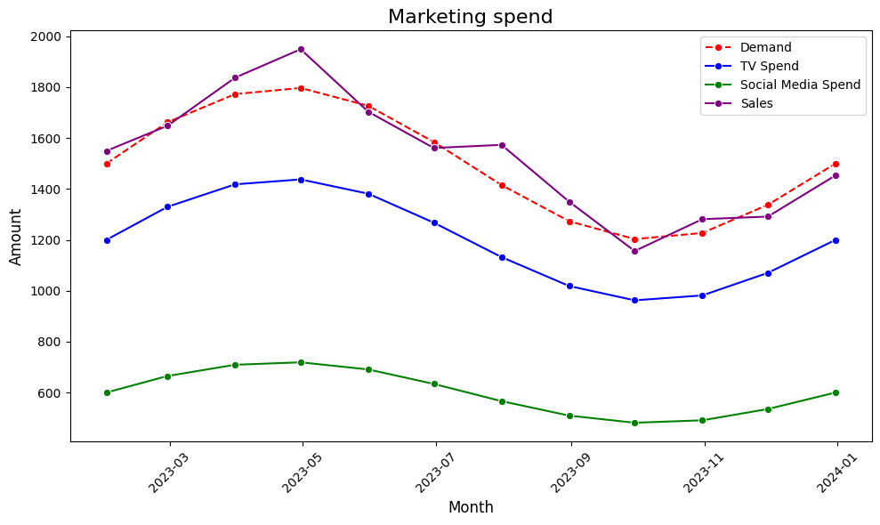
Let’s take an example from marketing. You sell a product where demand is highly seasonal — therefore, it makes sense to spend more on marketing during peak periods when demand is high. However, if both TV and social media spend follow the same seasonal pattern, it becomes difficult for the model to accurately determine the individual contribution of each channel.

Why is it a problem in causal inference?

Multi-collinearity can lead to the coefficients of the correlated variables becoming unstable and biased. When multi-collinearity is present, the standard errors of the regression coefficients tend to inflate. This means that the uncertainty around the estimates increases, making it harder to tell if a variable is truly significant.

Let’s go back to our marketing example, even if TV advertising and social media both drive sales, the model might struggle to separate their impacts because the inflated standard errors make the coefficient estimates unreliable.

We can simulate some examples in python to get a better understanding:

Example 1 — Marketing spend on each channel is equal, resulting in biased coefficients:

# Example 1 - marketing spend on each channel is equal: biased coefficients
np.random.seed(150)

tv_spend = np.random.normal(0, 50, 1000)
social_spend = tv_spend
sales = 0.10 * tv_spend + 0.20 * social_spend
X = np.column_stack((tv_spend, social_spend))
clf = LinearRegression()
clf.fit(X, sales)

print(f'Coefficients: {clf.coef_}')

Example 2 — Marketing spend on each channel follows the same trend, this time resulting in a coefficient sign flip:

# Example 2 - marketing spend on each channel follows the same trend: biased coefficients and sign flip
np.random.seed(150)

tv_spend = np.random.normal(0, 50, 1000)
social_spend = tv_spend * 0.50
sales = 0.10 * tv_spend + 0.20 * social_spend
X = np.column_stack((tv_spend, social_spend))
clf = LinearRegression()
clf.fit(X, sales)

print(f'Coefficients: {clf.coef_}')

Example 3 — The addition of random noise allows the model to estimate the correct coefficients:

# Example 3 - random noise added to marketing spend: correct coefficients
np.random.seed(150)

tv_spend = np.random.normal(0, 50, 1000)
social_spend = tv_spend * 0.50 + np.random.normal(0, 1, 1000)
sales = 0.10 * tv_spend + 0.20 * social_spend
X = np.column_stack((tv_spend, social_spend))
clf = LinearRegression()
clf.fit(X, sales)

print(f'Coefficients: {clf.coef_}')

Additionally, multi-collinearity can cause a phenomenon known as sign flipping, where the direction of the effect (positive or negative) of a variable can reverse unexpectedly. For instance, even though you know social media advertising should positively impact sales, the model might show a negative coefficient simply because of its high correlation with TV spend. We can see this in example 2.

Why is it so common in marketing mix modelling?

We’ve already touched upon one key issue: marketing teams often have a strong understanding of demand patterns and use this knowledge to set budgets. Typically, they increase spending across multiple channels during peak demand periods. While this makes sense from a strategic perspective, it can inadvertently create a multi-collinearity problem.

Even for products where demand is fairly constant, if the marketing team upweight or downweight each channel by the same percentage each week/month, then this will also leave us with a multi-collinearity problem.

The other reason I’ve seen for multi-collinearity in MMM is poorly specified causal graphs (DAGs). If we just throw everything into a flat regression, it’s likely we will have a multi-collinearity problem. Take the example below — If paid search impressions can be explained using TV and Social spend, then including it alongside TV and Social in a flat linear regression model is likely going to lead to multi-collinearity.

How can we detect it?

Detecting multi-collinearity is crucial to prevent it from skewing causal inferences. Here are some common methods to identify it:

Correlation

A simple and effective way to detect multi-collinearity is by examining the correlation matrix. This matrix shows pairwise correlations between all variables in the dataset. If two predictors have a correlation coefficient close to +1 or -1, they are highly correlated, which could indicate multi-collinearity.

Variance inflation factor (VIF)

Quantifies how much the variance of a regression coefficient is inflated due to multi-collinearity:

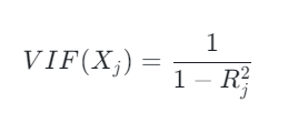
The R-squared is obtained by regressing all of the other independent variables on the chosen variable. If the R-squared is high this means the chosen variable can be predicted using the other independent variables (which results in a high VIF for the chosen variable).

There are some rule-of-thumb cut-offs for VIF in terms of detecting multi-collinearity – However, i’ve not found any convincing resources backing them up so I will not quote them here.

Standard errors

The standard error of a regression coefficient tells you how precisely that coefficient is estimated. It is calculated as the square root of the variance of the coefficient estimate. High standard errors may indicate multi-collinearity.

Simulations

Also the knowing the 3 approaches highlighted above is useful, it can still be hard to quantify whether you have a serious problem with multi-collinearity. Another approach you could take is running a simulation with known coefficients and then seeing how well you can estimate them with your model. Let’s illustrate using an MMM example:

• Extract channel spend and sales data as normal.

-- example SQL code to extract data
select
  observation_date,
  sum(tv_spend) as tv_spend,
  sum(social_spend) as social_spend,
  sum(sales) as sales
from mmm_data_mart
group by
  observation_date;

• Create data generating process, setting a coefficient for each channel.

# set coefficients for each channel using actual spend data
marketing_contribution = tv_spend * 0.10 + social_spend * 0.20

# calculate the remaining contribution
other_contribution = sales - marketing_contribution

# create arrays for regression
X = np.column_stack((tv_spend, social_spend, other_contribution))
y = sales

• Train model and compare estimated coefficients to those set in the last step.

# train regression model
clf = LinearRegression()
clf.fit(X, y)

# recover coefficients
print(f'Recovered coefficients: {clf.coef_}')

Now we know how we can identify multi-collinearity, let’s move on and explore how we can address it!

How can we address it?

There are several strategies to address multi-collinearity:

1. Removing one of the correlated variables
   This is a straightforward way to reduce redundancy. However, removing a variable blindly can be risky — especially if the removed variable is a confounder. A helpful step is determining the causal graph (DAG). Understanding the causal relationships allows you to assess whether dropping a correlated variable still enables valid inferences.
2. Combining variables
   When two or more variables provide similar information, you can combine them. This method reduces the dimensionality of the model, mitigating multi-collinearity risk while preserving as much information as possible. As with the previous approach, understanding the causal structure of the data is crucial.
3. Regularization techniques
   Regularization methods such as Ridge or Lasso regression are powerful tools to counteract multi-collinearity. These techniques add a penalty to the model’s complexity, shrinking the coefficients of correlated predictors. Ridge focuses on reducing the magnitude of all coefficients, while Lasso can drive some coefficients to zero, effectively selecting a subset of predictors.
4. Bayesian priors
   Using Bayesian regression techniques, you can introduce prior distributions for the parameters based on existing knowledge. This allows the model to “regularize” based on these priors, reducing the impact of multi-collinearity. By informing the model about reasonable ranges for parameter values, it prevents overfitting to highly correlated variables. We’ll delve into this method in the case study to illustrate its effectiveness.
5. Random budget adjustments
   Another strategy, particularly useful in marketing mix modeling (MMM), is introducing random adjustments to your marketing budgets at a channel level. By systematically altering the budgets you can start to observe the isolated effects of each. There are two main challenges with this method (1) Buy-in from the marketing team and (2) Once up and running it could take months or even years to collect enough data for your model. We will also cover this one off in the case study with some simulations.

We will test some of these strategies out in the case study next.

An introduction to Bayesian priors

A deep dive into Bayesian priors is beyond the scope of this article, but let’s cover some of the intuition behind them to ensure we can follow the case study.

Bayesian priors represent our initial beliefs about the values of parameters before we observe any data. In a Bayesian approach, we combine these priors with actual data (via a likelihood function) to update our understanding and calculate the posterior distribution, which reflects both the prior information and the data.

To simplify: when building an MMM, we need to feed the model some prior beliefs about the coefficients of each variable. Instead of supplying a fixed upper and lower bound, we provide a distribution. The model then searches within this distribution and, using the data, calculates the posterior distribution. Typically, we use the mean of this posterior distribution to get our coefficient estimates.

Of course, there’s more to Bayesian priors than this, but the explanation above serves as a solid starting point!

Case study

You’ve recently joined a start-up who have been running their marketing strategy for a couple of years now. They want to start measuring it using MMM, but their early attempts gave unintuitive results (TV had a negative contribution!). It seems their problem stems from the fact that each marketing channel owner is setting their budget based on the demand forecast, leading to a problem with multi-collinearity. You are tasked with assessing the situation and recommending next steps.

Data-generating-process

Let’s start by creating a data-generating function in python with the following properties:

• Demand is made up of 3 components: trend, seasonality and noise.
• The demand forecast model comes from the data science team and can accurately predict within +/- 5% accuracy.
• This demand forecast is used by the marketing team to set the budget for social and TV spend — We can add some random variation to these budgets using the spend_rand_change parameter.
• The marketing team spend twice as much on TV compared to social media.
• Sales are driven by a linear combination of demand, social media spend and TV spend.
• The coefficients for social media and TV spend can be set using the true_coef parameter.

def data_generator(spend_rand_change, true_coef):
    '''
    Generate simulated marketing data with demand, forecasted demand, social and TV spend, and sales.

    Args:
        spend_rand_change (float): Random variation parameter for marketing spend.
    true_coef (list): True coefficients for demand, social media spend, and TV spend effects on sales.

    Returns:
        pd.DataFrame: DataFrame containing the simulated data.
    '''
    
    # Parameters for data generation
    start_date = "2018-01-01"
    periods = 365 * 3  # Daily data for three years
    trend_slope = 0.01  # Linear trend component
    seasonal_amplitude = 5  # Amplitude of the seasonal component
    seasonal_period = 30.44  # Monthly periodicity
    noise_level = 5  # Level of random noise in demand

    # Generate time variables
    time = np.arange(periods)
    date_range = pd.date_range(start=start_date, periods=periods)

    # Create demand components
    trend_component = trend_slope * time
    seasonal_component = seasonal_amplitude * np.sin(2 * np.pi * time / seasonal_period)
    noise_component = noise_level * np.random.randn(periods)

    # Combine to form demand series
    demand = 100 + trend_component + seasonal_component + noise_component

    # Initialize DataFrame
    df = pd.DataFrame({'date': date_range, 'demand': demand})

    # Add forecasted demand with slight random variation
    df['demand_forecast'] = df['demand'] * np.random.uniform(0.95, 1.05, len(df))

    # Simulate social media and TV spend with random variation
    df['social_spend'] = df['demand_forecast'] * 10 * np.random.uniform(1 - spend_rand_change, 1 + spend_rand_change, len(df))
    df['tv_spend'] = df['demand_forecast'] * 20 * np.random.uniform(1 - spend_rand_change, 1 + spend_rand_change, len(df))
    df['total_spend'] = df['social_spend'] + df['tv_spend']

    # Calculate sales based on demand, social, and TV spend, with some added noise
    df['sales'] = (
        df['demand'] * true_coef[0] + 
        df['social_spend'] * true_coef[1] + 
        df['tv_spend'] * true_coef[2]
    )
    sales_noise = 0.01 * df['sales'] * np.random.randn(len(df))
    df['sales'] += sales_noise
    
    return df

Initial assessment

Now let’s simulate some data with no random variation applied to how the marketing team set the budget — We will try and estimate the true coefficients. The function below is used to train the regression model:

def run_reg(df, features, target):
    '''
    Runs a linear regression on the specified features to predict the target variable.

    Args:
        df (pd.DataFrame): The input data containing features and target.
    features (list): List of column names to be used as features in the regression.
    target (str): The name of the target column to be predicted.
    Returns:
        np.ndarray: Array of recovered coefficients from the linear regression model.
    '''
    
    # Extract features and target values
    X = df[features].values
    y = df[target].values

    # Initialize and fit linear regression model
    model = LinearRegression()
    model.fit(X, y)

    # Output recovered coefficients
    coefficients = model.coef_
    print(f'Recovered coefficients: {coefficients}')
    
    return coefficients

np.random.seed(40)

true_coef = [0.35, 0.15, 0.05]

features = [
    "demand",
    "social_spend",
    "tv_spend"
]

target = "sales"

sim_1 = data_generator(0.00, true_coef)
reg_1 = run_reg(sim_1, features, target)

print(f"True coefficients: {true_coef}")

We can see that the coefficient for social spend is underestimated whilst the coefficient for tv spend is overestimated. Good job you didn’t give the marketing team this model to optimise their budgets — It would have ended in disaster!

In the short-term, could using Bayesian priors give less biased coefficients?

In the long-term, would random budget adjustments create a dataset which doesn’t suffer from multi-collinearity?

Let’s try and find out!

Bayesian priors

Let’s start with exploring Bayesian priors…

We will be using my favourite MMM implementation pymc marketing:

Guide – pymc-marketing 0.8.0 documentation

We will use the same data we generated in the initial assessment:

date_col = "date"

y_col = "sales"

channel_cols = ["social_spend",
                "tv_spend"]

control_cols = ["demand"]

X = sim_1[[date_col] + channel_cols + control_cols]
y = sim_1[y_col]

Before we get into the modelling lets have a look at the contribution for each variable:

# calculate contribution
true_contributions = [round(np.sum(X["demand"] * true_coef[0]) / np.sum(y), 2), 
                      round(np.sum(X["social_spend"] * true_coef[1]) / np.sum(y), 2), 
                      round(np.sum(X["tv_spend"] * true_coef[2]) / np.sum(y), 2)]
true_contributions

Bayesian (default) priors

Let’s see what result we get if we use the default priors. Below you can see that there are a lot of priors! This is because we have to supply priors for the intercept, ad stock and saturation transformation amongst other things. It’s the saturation beta we are interested in – This is the equivalent of the variable coefficients we are trying to estimate.

mmm_default = MMM(
    adstock="geometric",
    saturation="logistic",
    date_column=date_col,
    channel_columns=channel_cols,
    control_columns=control_cols,
    adstock_max_lag=4,
    yearly_seasonality=2,
)

mmm_default.default_model_config

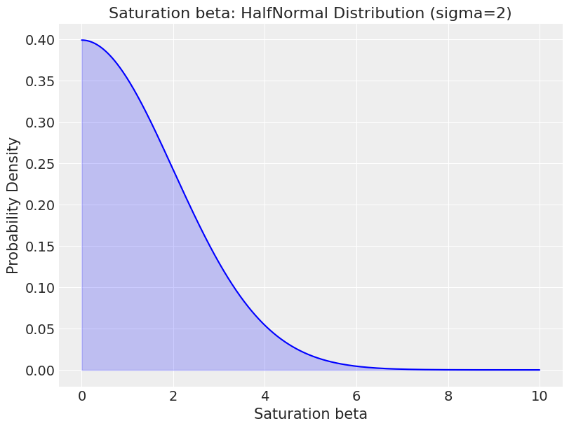
We have to supply a distribution. The HalfNormal is a sensible choice for channel coefficients as we know they can’t be negative. Below we visualise what the distribution looks like to bring it to life:

sigma = 2

x1 = np.linspace(0, 10, 1000)
y1 = halfnorm.pdf(x1, scale=sigma)

plt.figure(figsize=(8, 6))
plt.plot(x1, y1, 'b-')
plt.fill_between(x1, y1, alpha=0.2, color='blue')
plt.title('Saturation beta: HalfNormal Distribution (sigma=2)')
plt.xlabel('Saturation beta')
plt.ylabel('Probability Density')
plt.grid(True)
plt.show()

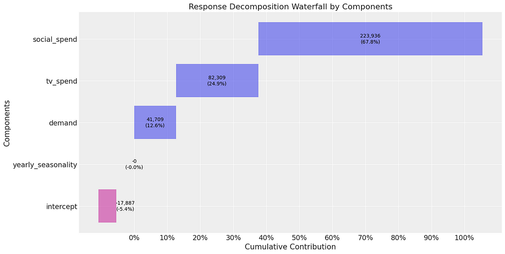
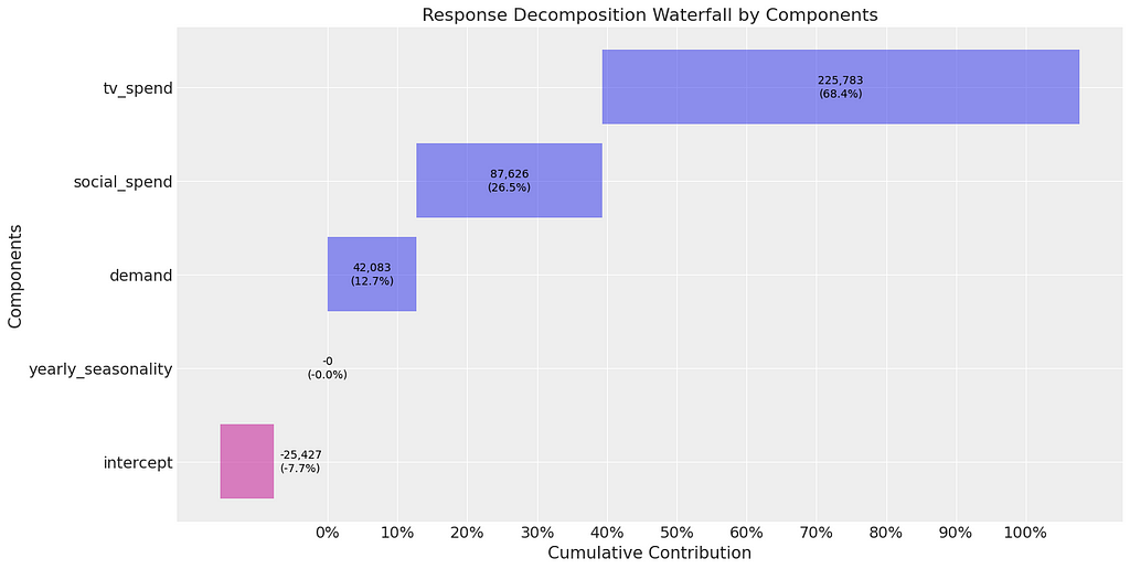
Now we are ready to train the model and extract the contributions of each channel. As before our coefficients are biased (we know this as the contributions for each channel aren’t correct — social media should be 50% and TV should be 35%). However, interestingly they are much closer to the true contribution compared to when we ran linear regression before. This would actually be a reasonable starting point for the marketing team!

mmm_default.fit(X, y)
mmm_default.plot_waterfall_components_decomposition();

Bayesian (custom) priors

Before we move on, let’s take the opportunity to think about custom priors. One (very bold) assumption we can make is that each channel has a similar return on investment (or in our case where we don’t have revenue, cost per sale). We can therefore use the spend distribution across channel to set some custom priors.

As the MMM class does feature scaling in both the target and features, priors also need to be supplied in the scaled space. This actually makes it quite easy for us to do as you can see in the below code:

total_spend_per_channel = df[channel_cols].sum(axis=0)
spend_share = total_spend_per_channel / total_spend_per_channel.sum()

n_channels = df[channel_cols].shape[1]
prior_sigma = n_channels * spend_share.to_numpy()

spend_share

We then need to feed the custom priors into the model.

my_model_config = {'saturation_beta': {'dist': 'HalfNormal', 'kwargs': {'sigma': prior_sigma}}}

mmm_priors = MMM(
    model_config=my_model_config,
    adstock="geometric",
    saturation="logistic",
    date_column=date_col,
    channel_columns=channel_cols,
    control_columns=control_cols,
    adstock_max_lag=4,
    yearly_seasonality=2,
)

mmm_priors.default_model_config

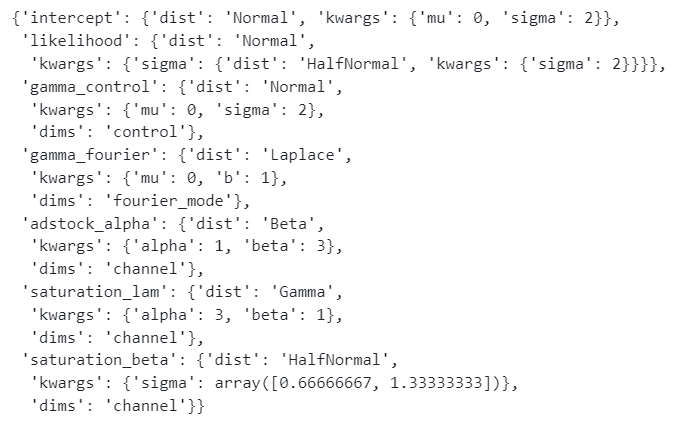
When we train the model and extract the coefficients we see that the priors have come into play, with tv now having the highest contribution (because we spent more than social). However, this is very wrong and illustrates why we have to be so careful when setting priors! The marketing team should really think about running some experiments to help them set priors.

mmm_priors.fit(X, y)
mmm_priors.plot_waterfall_components_decomposition();

Random budget adjustments

Now we have our short-term plan in place, let’s think about the longer term plan. If we could persuade the marketing team to apply small random adjustments to their marketing channel budgets each month, would this create a dataset without multi-collinearity?

The code below uses the data generator function and simulates a range of random spend adjustments:

np.random.seed(40)

# Define list to store results
results = []

# Loop through a range of random adjustments to spend
for spend_rand_change in np.arange(0.00, 0.05, 0.001):
    # Generate simulated data with the current spend_rand_change
    sim_data = data_generator(spend_rand_change, true_coef)
    
    # Run the regression
    coefficients = run_reg(sim_data, features=['demand', 'social_spend', 'tv_spend'], target='sales')
    
    # Store the spend_rand_change and coefficients for later plotting
    results.append({
        'spend_rand_change': spend_rand_change,
        'coef_demand': coefficients[0],
        'coef_social_spend': coefficients[1],
        'coef_tv_spend': coefficients[2]
    })

# Convert results to DataFrame for easy plotting
results_df = pd.DataFrame(results)

# Plot the coefficients as a function of spend_rand_change
plt.figure(figsize=(10, 6))
plt.plot(results_df['spend_rand_change'], results_df['coef_demand'], label='Demand Coef', color='r', marker='o')
plt.plot(results_df['spend_rand_change'], results_df['coef_social_spend'], label='Social Spend Coef', color='g', marker='o')
plt.plot(results_df['spend_rand_change'], results_df['coef_tv_spend'], label='TV Spend Coef', color='b', marker='o')

# Add lines for the true coefficients
plt.axhline(y=true_coef[0], color='r', linestyle='--', label='True Demand Coef')
plt.axhline(y=true_coef[1], color='g', linestyle='--', label='True Social Spend Coef')
plt.axhline(y=true_coef[2], color='b', linestyle='--', label='True TV Spend Coef')

plt.title('Regression Coefficients vs Spend Random Change')
plt.xlabel('Spend Random Change')
plt.ylabel('Coefficient Value')
plt.legend()
plt.grid(True)
plt.show()

We can see from the results that just a small random adjustment to the budget for each channel can break free of the multi-collinearity curse!

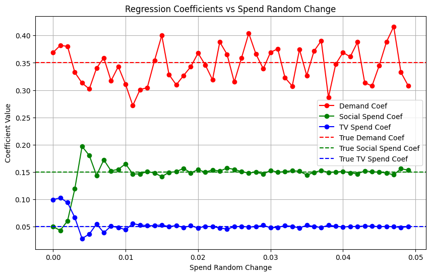
It’s worth noting that if I change the random seed (almost like resampling), the starting point for the coefficients varies — However, whatever seed I used the coefficients stabilised after a 1% random change in spend. I’m sure this will vary depending on your data-generating process so make sure you test it out using your own data!

Final thoughts

• Although the focus of this article was multi-collinearity, the big take away is the importance of simulating data and then trying to estimate the known coefficients (remember you set them yourself so you know them) — It’s an essential step if you want to have confidence in your results!
• When it comes to MMM, it can be useful to use your actual spend and sales data as the base for your simulation — This will help you understand if you have a multi-collinearity problem.
• If you use actual spend and sales data you can also carry out a random budget adjustment simulation to help come up with a suitable randomisation strategy for the marketing team. Keep in mind my simulation was simplistic to illustrate a point — We could design a much more effective strategy e.g. testing different areas of the response curve for each channel.
• Bayesian can be a steep learning curve — The other approach we could take is using a constrained regression in which you set upper and lower bounds for each channel coefficient based on prior knowledge.
• If you are setting Bayesian priors, it’s super important to be transparent about how they work and how they were selected. If you go down the route of using the channel spend distribution, the assumption that each channel has a similar ROI needs signing off from the relevant stakeholders.
• Bayesian priors are not magic! Ideally you would use results from experiments to set your priors — It’s worth checking out how the pymc marketing have approached this:

Lift Test Calibration – pymc-marketing 0.8.0 documentation

That is it, hope you enjoyed this instalment! Follow me if you want to continue this journey into Causal AI – In the next article we will immerse ourselves in the topic of bad controls!

Is Multi-Collinearity Destroying Your Causal Inferences In Marketing Mix Modelling? was originally published in Towards Data Science on Medium, where people are continuing the conversation by highlighting and responding to this story.