How to Use Elastic Net Regression

Cast a flexible net that only retains big fish

Note: The code used in this article utilizes three custom scripts, data_cleaning, data_review, and , eda, that can be accessed through a public GitHub repository.

It is like a stretchable fishing net that retains ‘all the big fish’ Zou & Hastie (2005) p. 302

Background

Linear regression is a commonly used teaching tool in data science and, under the appropriate conditions (e.g., linear relationship between the independent and dependent variables, absence of multicollinearity), it can be an effective method for predicting a response. However, in some scenarios (e.g., when the model’s structure becomes complex), its use can be problematic.

To address some of the algorithm’s limitations, penalization or regularization techniques have been suggested [1]. Two popular methods of regularization are ridge and lasso regression, but choosing between these methods can be difficult for those new to the field of data science.

One approach to choosing between ridge and lasso regression is to examine the relevancy of the features to the response variable [2]. When the majority of features in the model are relevant (i.e., contribute to the predictive power of the model), the ridge regression penalty (or L2 penalty) should be added to linear regression.

When the ridge regression penalty is added, the cost function of the model is:

• θ = the vector of parameters or coefficients of the model
• α = the overall strength of the regularization
• m = the number of training examples
• n = the number of features in the dataset

When the majority of features are irrelevant (i.e., do not contribute to the predictive power of the model), the lasso regression penalty (or L1 penalty) should be added to linear regression.

When the lasso regression penalty is added, the cost function of the model is:

Relevancy can be determined through manual review or cross validation; however, when working with several features, the process becomes time consuming and computationally expensive.

An efficient and flexible solution to this issue is using elastic net regression, which combines the ridge and lasso penalties.

The cost function for elastic net regression is:

• r = the mixing ratio between ridge and lasso regression.

When r is 1, only the lasso penalty is used and when r is 0 , only the ridge penalty is used. When r is a value between 0 and 1, a mixture of the penalties is used.

In addition to being well-suited for datasets with several features, elastic net regression has other attributes that make it an appealing tool for data scientists [1]:

• Automatic selection of relevant features, which results in parsimonious models that are easy to interpret
• Continuous shrinkage, which gradually reduces the coefficients of less relevant features towards zero (opposed to an immediate reduction to zero)
• Ability to select groups of correlated features, instead of selecting one feature from the group arbitrarily

Due to its utility and flexibility, Zou and Hastie (2005) compared the model to a “…stretchable fishing net that retains all the big fish.” (p. 302), where big fish are analogous to relevant features.

Now that we have some background, we can move forward to implementing elastic net regression on a real dataset.

Implementation

A great resource for data is the University of California at Irvine’s Machine Learning Repository (UCI ML Repo). For the tutorial, we’ll use the Wine Quality Dataset [3], which is licensed under a Creative Commons Attribution 4.0 International license.

The function displayed below can be used to obtain datasets and variable information from the UCI ML Repo by entering the identification number as the parameter of the function.

pip install ucimlrepo # unless already installed

from ucimlrepo import fetch_ucirepo
import pandas as pd

def fetch_uci_data(id):
    """
    Function to return features datasets from the UCI ML Repository.

    Parameters
    ----------
    id: int
        Identifying number for the dataset

    Returns
    ----------
    df: df
        Dataframe with features and response variable 
    """
    dataset = fetch_ucirepo(id=id) 

    features = pd.DataFrame(dataset.data.features)
    response = pd.DataFrame(dataset.data.targets)
    df = pd.concat([features, response], axis=1)
    
    # Print variable information
    print('Variable Information')
    print('--------------------')
    print(dataset.variables)

    return(df)

# Wine Quality's identification number is 186
df = fetch_uci_data(186)

A pandas dataframe has been assigned to the variable “df” and information about the dataset has been printed.

Exploratory Data Analysis

Variable Information
--------------------
                    name     role         type demographic  
0          fixed_acidity  Feature   Continuous        None   
1       volatile_acidity  Feature   Continuous        None   
2            citric_acid  Feature   Continuous        None   
3         residual_sugar  Feature   Continuous        None   
4              chlorides  Feature   Continuous        None   
5    free_sulfur_dioxide  Feature   Continuous        None   
6   total_sulfur_dioxide  Feature   Continuous        None   
7                density  Feature   Continuous        None   
8                     pH  Feature   Continuous        None   
9              sulphates  Feature   Continuous        None   
10               alcohol  Feature   Continuous        None   
11               quality   Target      Integer        None   
12                 color    Other  Categorical        None   

               description units missing_values  
0                     None  None             no  
1                     None  None             no  
2                     None  None             no  
3                     None  None             no  
4                     None  None             no  
5                     None  None             no  
6                     None  None             no  
7                     None  None             no  
8                     None  None             no  
9                     None  None             no  
10                    None  None             no  
11  score between 0 and 10  None             no  
12            red or white  None             no

Based on the variable information, we can see that there are 11 “features”, 1 “target”, and 1 “other” variables in the dataset. This is interesting information — if we had extracted the data without the variable information, we may not have known that there were data available on the family (or color) of wine. At this time, we won’t be incorporating the “color” variable into the model, but it’s nice to know it’s there for future iterations of the project.

The “description” column in the variable information suggests that the “quality” variable is categorical. The data are likely ordinal, meaning they have a hierarchical structure but the intervals between the data are not guaranteed to be equal or known. In practical terms, it means a wine rated as 4 is not twice as good as a wine rated as 2. To address this issue, we’ll convert the data to the proper data-type.

df['quality'] = df['quality'].astype('category')

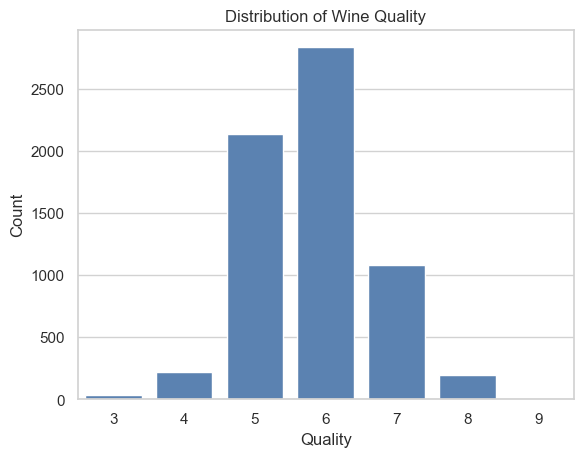
To gain a better understanding of the data, we can use the countplot() method from the seaborn package to visualize the distribution of the “quality” variable.

import seaborn as sns
import matplotlib.pyplot as plt 

sns.set_theme(style='whitegrid') # optional

sns.countplot(data=df, x='quality')
plt.title('Distribution of Wine Quality')
plt.xlabel('Quality')
plt.ylabel('Count')
plt.show()

When conducting an exploratory data analysis, creating histograms for numeric features is beneficial. Additionally, grouping the variables by a categorical variable can provide new insights. The best option for grouping the data is “quality”. However, given there are 7 groups of quality, the plots could become difficult to read. To simplify grouping, we can create a new feature, “rating”, that organizes the data on “quality” into three categories: low, medium, and high.

def categorize_quality(value):
 if 0 <= value <= 3:
    return 0 # low rating
 elif 4 <= value <= 6:
    return 1 # medium rating
 else:
    return # high rating

# Create new column for 'rating' data
df['rating'] = df['quality'].apply(categorize_quality)

To determine how many wines are each group, we can use the following code:

df['rating'].value_counts()

rating
1    5190
2    1277
0      30
Name: count, dtype: int64

Based on the output of the code, we can see that the majority of wines are categorized as “medium”.

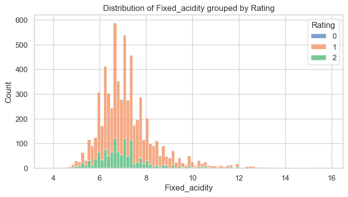
Now, we can plot histograms of the numeric features groups by “rating”. To plot the histogram we’ll need to use the gen_histograms_by_category() method from the eda script in the GitHub repository shared at the beginning of the article.

import eda 

eda.gen_histograms_by_category(df, 'rating')

Above is one of the plots generated by the method. A review of the plot indicates there is some skew in the data. To gain a more precise measure of skew, along with other statistics, we can use the get_statistics() method from the data_review script.

from data_review import get_statistics

get_statistics(df)

-------------------------
Descriptive Statistics
-------------------------
          fixed_acidity  volatile_acidity  citric_acid  residual_sugar    chlorides  free_sulfur_dioxide  total_sulfur_dioxide      density           pH    sulphates      alcohol      quality
count       6497.000000       6497.000000  6497.000000     6497.000000  6497.000000          6497.000000           6497.000000  6497.000000  6497.000000  6497.000000  6497.000000  6497.000000
mean           7.215307          0.339666     0.318633        5.443235     0.056034            30.525319            115.744574     0.994697     3.218501     0.531268    10.491801     5.818378
std            1.296434          0.164636     0.145318        4.757804     0.035034            17.749400             56.521855     0.002999     0.160787     0.148806     1.192712     0.873255
min            3.800000          0.080000     0.000000        0.600000     0.009000             1.000000              6.000000     0.987110     2.720000     0.220000     8.000000     3.000000
25%            6.400000          0.230000     0.250000        1.800000     0.038000            17.000000             77.000000     0.992340     3.110000     0.430000     9.500000     5.000000
50%            7.000000          0.290000     0.310000        3.000000     0.047000            29.000000            118.000000     0.994890     3.210000     0.510000    10.300000     6.000000
75%            7.700000          0.400000     0.390000        8.100000     0.065000            41.000000            156.000000     0.996990     3.320000     0.600000    11.300000     6.000000
max           15.900000          1.580000     1.660000       65.800000     0.611000           289.000000            440.000000     1.038980     4.010000     2.000000    14.900000     9.000000
skew           1.723290          1.495097     0.471731        1.435404     5.399828             1.220066             -0.001177     0.503602     0.386839     1.797270     0.565718     0.189623
kurtosis       5.061161          2.825372     2.397239        4.359272    50.898051             7.906238             -0.371664     6.606067     0.367657     8.653699    -0.531687     0.23232

Consistent with the histogram, the feature labeled “fixed_acidity” has a skewness of 1.72 indicating significant right-skewness.

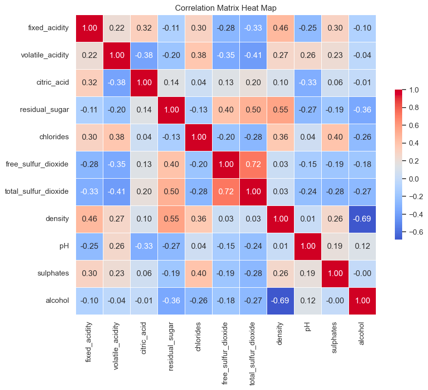
To determine if there are correlations between the variables, we can use another function from the eda script.

eda.gen_corr_matrix_hmap(df)

Although there a few moderate and strong relationships between features, elastic net regression performs well with correlated variables, therefore, no action is required [2].

Data Cleaning

For the elastic net regression algorithm to run correctly, the numeric data must be scaled and the categorical variables must be encoded.

To clean the data, we’ll take the following steps:

1. Scale the data using the the scale_data() method from the the data_cleaning script
2. Encode the “quality” and “rating” variables using the the get_dummies() method from pandas
3. Separate the features (i.e., X) and response variable (i.e., y) using the separate_data() method
4. Split the data into train and test sets using train_test_split()

from sklearn.model_selection import train_test_split
from data_cleaning import scale_data, separate_data

df_scaled = scale_data(df)
df_encoded = pd.get_dummies(df_scaled, columns=['quality', 'rating'])

# Separate features and response variable (i.e., 'alcohol')
X, y = separate_data(df_encoded, 'alcohol')

# Create test and train sets 
X_train, X_test, y_train, y_test = train_test_split(X, y, test_size =0.2, random_state=0)

Model Building and Evaluation

To train the model, we’ll use ElasticNetCV() which has two parameters, alpha and l1_ratio, and built-in cross validation. The alpha parameter determines the strength of the regularization applied to the model and l1_ratio determines the mix of the lasso and ridge penalty (it is equivalent to the variable r that was reviewed in the Background section).

• When l1_ratio is set to a value of 0, the ridge regression penalty is used.
• When l1_ratio is set to a value of 1, the lasso regression penalty is used.
• When l1_ratio is set to a value between 0 and 1, a mixture of both penalties are used.

Choosing values for alpha and l1_ratio can be challenging; however, the task is made easier through the use of cross validation, which is built into ElasticNetCV(). To make the process easier, you don’t have to provide a list of values from alpha and l1_ratio — you can let the method do the heavy lifting.

from sklearn.linear_model import ElasticNet, ElasticNetCV

# Build the model
elastic_net_cv = ElasticNetCV(cv=5, random_state=1)

# Train the model
elastic_net_cv.fit(X_train, y_train)

print(f'Best Alpha: {elastic_net_cv.alpha_}')
print(f'Best L1 Ratio:{elastic_net_cv.l1_ratio_}')

Best Alpha: 0.0013637974514517563
Best L1 Ratio:0.5

Based on the printout, we can see the best values for alpha and l1_ratio are 0.001 and 0.5, respectively.

To determine how well the model performed, we can calculate the Mean Squared Error and the R-squared score of the model.

from sklearn.metrics import mean_squared_error

# Predict values from the test dataset
elastic_net_pred = elastic_net_cv.predict(X_test)

mse = mean_squared_error(y_test, elastic_net_pred)
r_squared = elastic_net_cv.score(X_test, y_test)

print(f'Mean Squared Error: {mse}')
print(f'R-squared value: {r_squared}')

Mean Squared Error: 0.2999434011721803
R-squared value: 0.7142939720612289

Conclusion

Based on the evaluation metrics, the model performs moderately well. However, its performance could be enhanced through some additional steps, like detecting and removing outliers, additional feature engineering, and providing a specific set of values for alpha and l1_ratio in ElasticNetCV(). Unfortunately, those steps are beyond the scope of this simple tutorial; however, they may provide some ideas for how this project could be improved by others.

Thank you for taking the time to read this article. If you have any questions or feedback, please leave a comment.

References

[1] H. Zou & T. Hastie, Regularization and Variable Selection Via the Elastic Net, Journal of the Royal Statistical Society Series B: Statistical Methodology, Volume 67, Issue 2, April 2005, Pages 301–320, https://doi.org/10.1111/j.1467-9868.2005.00503.x

[2] A. Géron, Hands-On Machine Learning with Scikit-Learn, Keras & Tensorflow: Concepts, Tools, and Techniques to Build Intelligent Systems (2021), O’Reilly.

[3] P. Cortez, A. Cerdeira, F. Almeida, T. Matos, & Reis,J.. (2009). Wine Quality. UCI Machine Learning Repository. https://doi.org/10.24432/C56S3T.

How to Use Elastic Net Regression was originally published in Towards Data Science on Medium, where people are continuing the conversation by highlighting and responding to this story.