How Neural Networks Learn: A Probabilistic Viewpoint

Understanding loss functions for training neural networks

Machine learning is very hands-on, and everyone charts their own path. There isn’t a standard set of courses to follow, as was traditionally the case. There’s no ‘Machine Learning 101,’ so to speak. However, this sometimes leaves gaps in understanding. If you’re like me, these gaps can feel uncomfortable. For instance, I used to be bothered by things we do casually, like the choice of a loss function. I admit that some practices are learned through heuristics and experience, but most concepts are rooted in solid mathematical foundations. Of course, not everyone has the time or motivation to dive deeply into those foundations — unless you’re a researcher.

I have attempted to present some basic ideas on how to approach a machine learning problem. Understanding this background will help practitioners feel more confident in their design choices. The concepts I covered include:

• Quantifying the difference in probability distributions using cross-entropy.
• A probabilistic view of neural network models.
• Deriving and understanding the loss functions for different applications.

Entropy

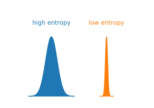
In information theory, entropy is a measure of the uncertainty associated with the values of a random variable. In other words, it is used to quantify the spread of distribution. The narrower the distribution the lower the entropy and vice versa. Mathematically, entropy of distribution p(x) is defined as;

It is common to use log with the base 2 and in that case entropy is measured in bits. The figure below compares two distributions: the blue one with high entropy and the orange one with low entropy.

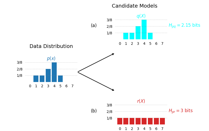
We can also measure entropy between two distributions. For example, consider the case where we have observed some data having the distribution p(x) and a distribution q(x) that could potentially serve as a model for the observed data. In that case we can compute cross-entropy Hpq​(X) between data distribution p(x) and the model distribution q(x). Mathematically cross-entropy is written as follows:

Using cross entropy we can compare different models and the one with lowest cross entropy is better fit to the data. This is depicted in the contrived example in the following figure. We have two candidate models and we want to decide which one is better model for the observed data. As we can see the model whose distribution exactly matches that of the data has lower cross entropy than the model that is slightly off.

There is another way to state the same thing. As the model distribution deviates from the data distribution cross entropy increases. While trying to fit a model to the data i.e. training a machine learning model, we are interested in minimizing this deviation. This increase in cross entropy due to deviation from the data distribution is defined as relative entropy commonly known as Kullback-Leibler Divergence of simply KL-Divergence.

Hence, we can quantify the divergence between two probability distributions using cross-entropy or KL-Divergence. To train a model we can adjust the parameters of the model such that they minimize the cross-entropy or KL-Divergence. Note that minimizing cross-entropy or KL-Divergence achieves the same solution. KL-Divergence has a better interpretation as its minimum is zero, that will be the case when the model exactly matches the data.

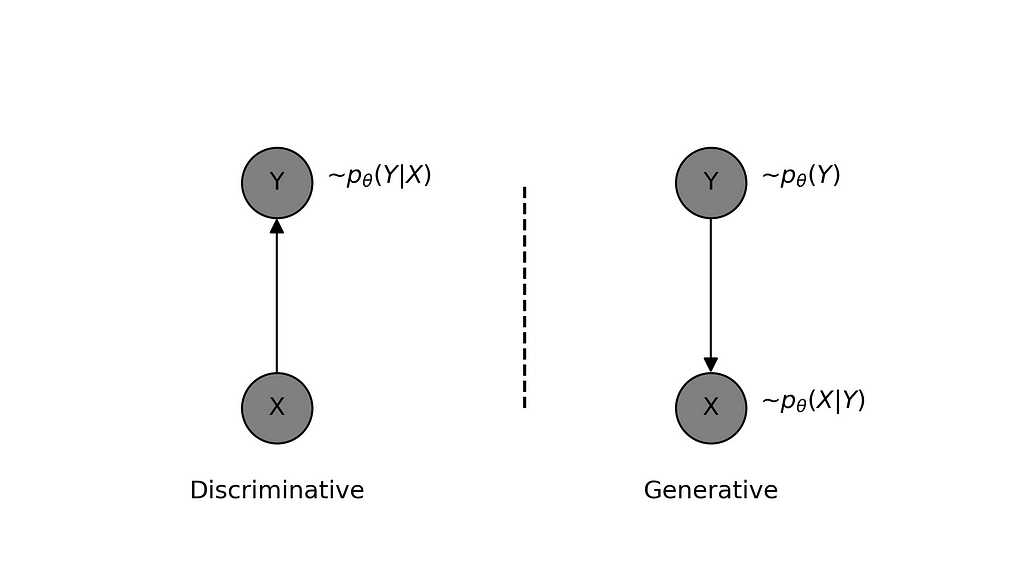
Another important consideration is how do we pick the model distribution? This is dictated by two things: the problem we are trying to solve and our preferred approach to solving the problem. Let’s take the example of a classification problem where we have (X, Y) pairs of data, with X representing the input features and Y representing the true class labels. We want to train a model to correctly classify the inputs. There are two ways we can approach this problem.

Discriminative vs Generative

The generative approach refers to modeling the joint distribution p(X,Y) such that it learns the data-generating process, hence the name ‘generative’. In the example under discussion, the model learns the prior distribution of class labels p(Y) and for given class label Y, it learns to generate features X using p(X|Y).

It should be clear that the learned model is capable of generating new data (X,Y). However, what might be less obvious is that it can also be used to classify the given features X using Bayes’ Rule, though this may not always be feasible depending on the model’s complexity. Suffice it to say that using this for a task like classification might not be a good idea, so we should instead take the direct approach.

Discriminative approach refers to modelling the relationship between input features X and output labels Y directly i.e. modelling the conditional distribution p(Y|X). The model thus learnt need not capture the details of features X but only the class discriminatory aspects of it. As we saw earlier, it is possible to learn the parameters of the model by minimizing the cross-entropy between observed data and model distribution. The cross-entropy for a discriminative model can be written as:

Where the right most sum is the sample average and it approximates the expectation w.r.t data distribution. Since our learning rule is to minimize the cross-entropy, we can call it our general loss function.

Goal of learning (training the model) is to minimize this loss function. Mathematically, we can write the same statement as follows:

Let’s now consider specific examples of discriminative models and apply the general loss function to each example.

Binary Classification

As the name suggests, the class label Y for this kind of problem is either 0 or 1. That could be the case for a face detector, or a cat vs dog classifier or a model that predicts the presence or absence of a disease. How do we model a binary random variable? That’s right — it’s a Bernoulli random variable. The probability distribution for a Bernoulli variable can be written as follows:

where π is the probability of getting 1 i.e. p(Y=1) = π.

Since we want to model p(Y|X), let’s make π a function of X i.e. output of our model π(X) depends on input features X. In other words, our model takes in features X and predicts the probability of Y=1. Please note that in order to get a valid probability at the output of the model, it has to be constrained to be a number between 0 and 1. This is achieved by applying a sigmoid non-linearity at the output.

To simplify, let’s rewrite this explicitly in terms of true label and predicted label as follows:

We can write the general loss function for this specific conditional distribution as follows:

This is the commonly referred to as binary cross entropy (BCE) loss.

Multi-class Classification

For a multi-class problem, the goal is to predict a category from C classes for each input feature X. In this case we can model the output Y as a categorical random variable, a random variable that takes on a state c out of all possible C states. As an example of categorical random variable, think of a six-faced die that can take on one of six possible states with each roll.

We can see the above expression as easy extension of the case of binary random variable to a random variable having multiple categories. We can model the conditional distribution p(Y|X) by making λ’s as function of input features X. Based on this, let’s we write the conditional categorical distribution of Y in terms of predicted probabilities as follows:

Using this conditional model distribution we can write the loss function using the general loss function derived earlier in terms of cross-entropy as follows:

This is referred to as Cross-Entropy loss in PyTorch. The thing to note here is that I have written this in terms of predicted probability of each class. In order to have a valid probability distribution over all C classes, a softmax non-linearity is applied at the output of the model. Softmax function is written as follows:

Regression

Consider the case of data (X, Y) where X represents the input features and Y represents output that can take on any real number value. Since Y is real valued, we can model the its distribution using a Gaussian distribution.

Again, since we are interested in modelling the conditional distribution p(Y|X). We can capture the dependence on X by making the conditional mean of Y a function of X. For simplicity, we set variance equal to 1. The conditional distribution can be written as follows:

We can now write our general loss function for this conditional model distribution as follows:

This is the famous MSE loss for training the regression model. Note that the constant factor is irrelevant here as we are only interest in finding the location of minima and can be dropped.

Summary

In this short article, I introduced the concepts of entropy, cross-entropy, and KL-Divergence. These concepts are essential for computing similarities (or divergences) between distributions. By using these ideas, along with a probabilistic interpretation of the model, we can define the general loss function, also referred to as the objective function. Training the model, or ‘learning,’ then boils down to minimizing the loss with respect to the model’s parameters. This optimization is typically carried out using gradient descent, which is mostly handled by deep learning frameworks like PyTorch. Hope this helps — happy learning!

How Neural Networks Learn: A Probabilistic Viewpoint was originally published in Towards Data Science on Medium, where people are continuing the conversation by highlighting and responding to this story.