How I Learned to Stop Worrying and Love the Partial Autocorrelation Coefficient

Beyond the obvious titular tribute to Dr. Strangelove, we’ll learn how to use the PACF to select the most influential regression variables with clinical precision

As a concept, the partial correlation coefficient is applicable to both time series and cross-sectional data. In time series settings, it’s often called the partial autocorrelation coefficient. In this article, I’ll focus more on the partial autocorrelation coefficient and its use in configuring Auto Regressive (AR) models for time-series data sets, particularly in the way it lets you weed out irrelevant regression variables from your AR model.

In the rest of the article, I’ll explain:

1. Why you need the partial correlation coefficient (PACF),
2. How to calculate the partial (auto-)correlation coefficient and the partial autocorrelation function,
3. How to determine if a partial (auto-)correlation coefficient is statistically significant, and
4. The uses of the PACF in building autoregressive time series models.

I will also explain how the concept of partial correlation can be applied to building linear models for cross-sectional data i.e. data that are not time-indexed.

A quick qualitative definition of partial correlation

Here’s a quick qualitative definition of partial correlation:

For linear models, the partial correlation coefficient of an explanatory variable x_k with the response variable y is the fraction of the linear correlation of x_k with y that is left over after the joint correlations of the rest of the variables with y acting either directly on y, or via x_k are eliminated, i.e. partialed out.

Don’t fret if that sounds like a mouthful. I’ll soon explain what it means, and illustrate the use of the partial correlation coefficient in detail using real-life data.

Let’s begin with a task that often vexes, confounds and ultimately derails some of the smartest regression model builders.

The troublesome task of selecting relevant regression variables

It’s one thing to select a suitable dependent variable that one wants to estimate. That’s often the easy part. It’s much harder to find explanatory variables that have the most influence on the dependent variable.

Let’s frame our problem in somewhat statistical terms:

Can you identify one or more explanatory variables whose variance explains much of the variance in the dependent variable?

For time series data, one often uses time-lagged copies of the dependent variable as explanatory variables. For example, if Y_t is the time-indexed dependent (a.k.a. response variable), a special linear regression model of the following kind known as an Autoregressive (AR) model can help us estimate Y_t.

In the above model, the explanatory variables are time-lagged copies of the dependent variables. Such models operate from the principle that the current value of a random variable is correlated with its previous values. In other words, the present is correlated with the past.

This is the point at which you will face a troublesome question: exactly how many lags of Y_t should you consider?

Which time-lags are the most relevant, the most influential, the most significant for explaining the variance in Y_t?

All too often, regression modelers rely — almost exclusively — on one of the following techniques for identifying the most influential regression variables.

• Stuff the regression model with all kinds of explanatory variables sometimes without the faintest idea of why a variable is being included. Then train the bloated model and pick out only those variables whose coefficients have a p value less than or equal to 0.05 i.e. ones which are statistically significant at a 95% confidence level. Now anoint these variables as the explanatory variables in a new (“final”) regression model.

OR when building a linear model, the following equally perilous technique:

• Select only those explanatory variables which have a) a linear relationship with the dependent variable and b) are also highly correlated with the dependent variable as measured by the Pearson’s coefficient coefficient.

Should you be seized with a urge to adopt these techniques, please do read the following first:

The trouble with the first technique is that stuffing your model with irrelevant variables makes the regression coefficients (the βs) lose their precision, meaning the confidence intervals of the estimated coefficients widen up. And what’s especially terrible about the loss of precision is that coefficients of all regression variables lose precision, not just the coefficients of the irrelevant variables. From this murky soup of impression, if you try to drain out the coefficients with high p values, there is a great chance you will throw out variables that are actually relevant.

Now let’s look at the second technique. You could scarcely guess the trouble with the second technique. The problem over there is even more insidious.

In many real-world situations, you would start with a list of candidate random variables that you are considering for adding to your model as explanatory variables. But often, many of these candidate variables are directly or indirectly correlated with each other. Thus, all variables as it were, exchange information with each other. The effect of this multi-way information exchange is that the correlation coefficient between a potential explanatory variable and the dependent variable hides within it, the correlations of other potential explanatory variables with the dependent variable.

For example, in a hypothetical linear regression model containing three explanatory variables, the correlation coefficient of the second variable with the dependent variable may contain a fraction of the joint correlation of the first and the third variables with the dependent variable that is acting via their joint correlation with the second variable.

Additionally, the joint correlation of the first and the third explanatory variable on the dependent variable also contributes to some of the correlation between the second explanatory variable and the dependent variable. This phenomenon arises from the fact that correlation between two variables is a perfectly symmetrical phenomenon.

Don’t worry if you feel a bit at sea from reading the above two paras. ThI will soon illustrate these indirect effects using a real-world data set, namely the El Niño Southern Oscillations data.

Sometimes, a substantial fraction of the correlation between a potential explanatory variable and the dependent variable is on account of other variables in the list of potential explanatory variables you are considering. If you go purely on the basis of the correlation coefficient’s value, you may accidentally select an irrelevant variable that is masquerading as a highly relevant variable under the false glow of a large correlation coefficient.

So how do you navigate around these troubles? For instance, in the Autoregressive model model shown above, how do you select the correct number of time lags p? Additionally, if your time series data exhibits seasonal behavior, how do you determine the seasonal order of your model?

The partial correlation coefficient gives you a powerful statistical instrument to answer these questions.

Using real-world time series data sets, we’ll develop the formula of the partial correlation coefficient and see how to put it to use for building an AR model for this data.

The Southern Oscillations Data set

The El Niño /Southern Oscillations (ENSO) data is a set of monthly observations of Sea Surface pressure (SSP). Each data point in the ENSO data set is the standardized difference in SSP observed at two points in the South Pacific that are 5323 miles apart, the two points being the tropical port city of Darwin in Australia and the Polynesian Island of Tahiti. Data points in the ENSO are one month apart. Meteorologists use the ENSO data to predict the onset of an El Niño or its opposite, the La Niña, event.

Here’s how the ENSO data looks like from January 1951 through May 2024:

Let Y_t be the value measured during month t, and Y_(t — 1) be the value measured during the previous month. As is often the case with time series data, Y_t and Y_(t — 1) might be correlated. Let’s find out.

A scatter plot of Y_t versus Y_(t — 1) brings out a strong linear (albeit heavily heteroskedastic) relationship between Y_t and Y_(t — 1).

We can quantify this linear relation using the Pearson’s correlation coefficient (r) between Y_t and Y_(t — 1). Pearson’s r is the ratio of the covariance between Y_t and Y_(t — 1) to the product of their respective standard deviations.

For the Southern Oscillations data, Pearson’s r between Y_t and Y_(t — 1) comes to out to be 0.630796 i.e. 63.08% which is a respectably large value. For reference, here is a matrix of correlations between different combinations of Y_t and Y_(t — k) where k goes from 0 to 10:

An AR(1) model for estimating the Differential SSP

Given the linear nature of the relation between Y_t and Y_(t — 1), a good first step toward estimating Y_t is to regress it on Y_(t — 1) using the following simple linear regression model:

The above model is called an AR(1) model. The (1) indicates that the maximum order of the lag is 1. As we saw earlier, the general AR(p) model is expressed as follows:

You will frequently build such autoregressive models while working with time series data.

Getting back to our AR(1) model, in this model, we hypothesize that some fraction of the variance in Y_t is explained by the variance in Y_(t — 1). What fraction is this? It’s exactly the value of the coefficient of determination R² (or more appropriately the adjusted-R²) of the fitted linear model.

The red dots in the figure below show the fitted AR(1) model and the corresponding R². I’ve included the Python code for generating this plot at the bottom of the article.

Making the case for Partial Autocorrelation Coefficient in autoregressive models

Let’s refer to the AR(1) model we constructed. The R² of this model is 0.40. So Y_(t — 1) and the intercept are able to together explain 40% of the variance in Y_t. Is it possible to explain some of the remaining 60% of variance in Y_t?

If you look at the correlation of Y_t with all of lagged copies of Y_t (see the highlighted column in the table below), you’ll see that practically every single one of them is correlated with Y_t by an amount that ranges from a substantial 0.630796 for Y_(t — 1) down to a non-trivial 0.076588 for Y_(t — 10).

In some wild moment of optimism, you may be tempted to stuff your regression model with all of these lagged variables which will turn your AR(1) model into an AR(10) model as follows:

But as I explained earlier, simply stuffing your model with all kinds of explanatory variables in the hope of getting a higher R² will be a grave folly.

The large correlations between Y_t and many of the lagged copies of Y_t can be deeply misleading. At least some of them are mirages that lure the R² thirsty model builder into certain statistical suicide.

So what’s driving the large correlations?

Here’s what is going on:

The correlation coefficient of Y_t with a lagged copy of itself such as Y_(t — k) consists of the following three components:

1. The joint correlation of Y_(t — 1), Y_(t — 2),…,Y_(t — k — 1) expressed directly with Y_t. Imagine a box that contains Y_(t — 1) , Y_(t — 2),…,Y_(t — k — 1). Now imagine a channel that transmits information about the contents of this box straight through to Y_t.
2. A fraction of the joint correlation of Y_(t — 1), Y_(t — 2),…,Y_(t— k — 1) that is expressed via the joint correlation of those three variables with Y_(t — k). Recall the imaginary box containing Y_(t — 1), Y_(t— 2),…,Y_(t — k — 1) . Now imagine a channel that transmits information about the contents of this box to Y_(t — k). Also imagine a second channel that transmits information about Y_(t— k) to Y_t. This second channel will also carry with it the information deposited at Y_(t — k) by the first channel.
3. The portion of the correlation of Y_t with Y_(t — k) that would be left over, were we to eliminate a.k.a. partial out the effects (1) and (2). What would be left over is the intrinsic correlation of Y_(t — k) with Y_t. This is the partial autocorrelation of Y_(t — k) with Y_t.

To illustrate, consider the correlation of Y_(t — 4) with Y_t. It’s 0.424304 or 42.43%.

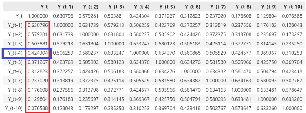
The correlation of Y_(t — 4) with Y_t arises from the following three information pathways:

1. The joint correlation of Y_(t — 1), Y_(t — 2) and Y_(t — 3) with Y_t expressed directly.
2. A fraction of the joint correlation of Y_(t — 1), Y_(t — 2) and Y_(t — 3) that is expressed via the joint correlation of those lagged variables with Y_(t — 4).
3. Whatever gets left over from 0.424304 when the effect of (1) and (2) is removed or partialed out. This “residue” is the intrinsic influence of Y_(t — 4) on Y_t which when quantified as a number in the [0, 1] range is called the partial correlation of Y_(t — 4) with Y_t.

Let’s bring out the essence of this discussion in slightly general terms:

In an autoregressive time series model of Y_t, the partial autocorrelation of Y_(t — k) with Y_t is the correlation of Y_(t — k) with Y_t that’s left over after the effect of all intervening lagged variables Y_(t — 1), Y_(t — 2),…,Y_(t — k — 1) is partialed out.

How to use the partial (auto-)correlation coefficient while creating an autoregressive time series model?

Consider the Pearson’s r of 0.424304 that Y_(t — 4) has with Y_t. As a regression modeler you’d naturally want to know how much of this correlation is Y_(t — 4)’s own influence on Y_t. If Y_(t — 4)’s own influence on Y_t is substantial, you’d want to include Y_(t — 4) as a regression variable in an autoregressive model for estimating Y_t.

But what if Y_(t — 4)’s own influence on Y_t is miniscule?

In that case, as far as estimating Y_t is concerned, Y_(t — 4) is an irrelevant random variable. You’d want to leave out Y_(t — 4) from your AR model as including an irrelevant variable will reduce the precision of your regression model.

Given these considerations, wouldn’t it be useful to know the partial autocorrelation coefficient of every single lagged value Y_(t — 1), Y_(t — 2), …, Y_(t — n) up to some n of interest? That way, you can precisely choose only those lagged variables that have a significant influence on the dependent variable in your AR model. The way to calculate these partial autocorrelations is by means of the partial autocorrelation function (PACF).

The partial autocorrelation function calculates the partial correlation of a time indexed variable with a time-lagged copy of itself for any time lag value you specify.

A plot of the PACF is a nifty way of quickly identifying the lags at which there is significant partial autocorrelation. Many Statistics libraries provide support for computing the PACF and for plotting the PACF. Following is the PACF plot I’ve created for Y_t (the ENSO index value for month t) using the plot_pacf function in the statsmodels.graphics.tsaplots Python package. See the bottom of this article for the source code.

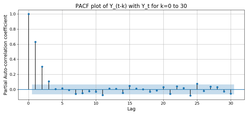
Let’s look at how to interpret this plot.

The sky blue rectangle around the X-axis is the 95% confidence interval for the null hypothesis that the partial correlation coefficients are not significant. You would consider only coefficients that lie outside — in practice, well outside — this blue sheath as statistically significant at a 95% confidence level.

The width of this confidence interval is calculated using the following formula:

In the above formula, z_α/2 is the value picked off from the standard normal N(0, 1) probability distribution. For e.g. for α=0.05 corresponding to a (1 — 0.05)100% = 95% confidence interval, the value of z_0.025 can be read off the standard normal distribution’s table as 1.96. The n in the denominator is the sample size. The smaller is your sample size, the wider is the interval and greater the probability that any given coefficient will lie within it rendering it statistically insignificant.

In the ENSO dataset, n is 871 observations. Plugging in z_0.025=1.96 and n=871, the width of the blue sheath for a 95% CI is:

[ — 1.96/√871, +1.96/√871] = [ — 0.06641, +0.06641]

You can see these extents clearly in a zoomed in view of the PACF plot:

Now let’s turn our attention to the correlations that are statistically significant.

The partial autocorrelation of Y_t at lag-0 (i.e. with itself) is always a perfect 1.0 since a random variable is always perfectly correlated with itself.

The partial autocorrelation at lag-1 is the simple autocorrelation of Y_t with Y_(t — 1) as there are no intervening variables between Y_t and Y_(t — 1). For the ENSO data set, this correlation is not only statistically significant, it’s also very high — in fact we saw earlier that it’s 0.424304.

Notice how the PACF cuts off sharply after k = 3:

A sharp cutoff at k=3 means that you must include exactly 3 time lags in your AR model as explanatory variables. Thus, an AR model for the ENSO data set is as follows:

Consider for a moment how incredibly useful to us has been the PACF plot.

• It’s informed us in clear and unmistakable terms what the exact number of lags (3) to use is for building the AR model for the ENSO data.
• It has given us the confidence to safely ignore all other lags, and
• It has greatly reduced the possibility of missing out important explanatory variables.

How to calculate the partial autocorrelation coefficient?

I’ll explain the calculation used in the PACF using the ENSO data. Recall for a moment the correlation of 0.424304 between Y_(t — 4) and Y_t. This is the simple (i.e. not partial) correlation between Y_(t — 4) and Y_t that we picked off from the table of correlations:

Recall also that this correlation is on account of the following correlation pathways:

1. The joint correlation of Y_(t — 1), Y_(t — 2) and Y_(t — 3) with Y_t expressed directly.
2. A fraction of the joint correlation of Y_(t — 1), Y_(t — 2) and Y_(t — 3) that is expressed via the joint correlation of those lagged variables with Y_(t — 4).
3. Whatever gets left over from 0.424304 when the effect of (1) and (2) is removed or partialed out. This “residue” is the intrinsic influence of Y_(t — 4) on Y_t which when quantified as a number in the [0, 1] range is called the partial correlation of Y_(t — 4) with Y_t.

To distill out the partial correlation, we must partial out effects (1) and (2).

How can we achieve this?

The following fundamental property of a regression model gives us a clever means to achieve our goal:

In a regression model of the type y = f(X) + e, the regression error (e) captures the balance amount of variance in the dependent variable (y) that the explanatory variables (X) aren’t able to explain.

We employ the above property using the following 3-step procedure:

Step-1

To partial out effect #1, we regress Y_t on Y_(t — 1), Y_(t — 2) and Y_(t — 3) as follows:

We train this model and capture the vector of residuals (ϵ_a) of the trained model. Assuming that the explanatory variables Y_(t — 1), Y_(t — 2) and Y_(t — 3) aren’t endogenous i.e. aren’t themselves correlated with the error term e_a of the model (if they are, then you have an altogether different sort of a problem to deal with!), the residuals ϵ_a from the trained model contain the fraction of the variance in Y_t that is not on account of the joint influence of Y_(t — 1), Y_(t — 2) and Y_(t — 3).

Here’s the training output showing the dependent variable Y_t, the explanatory variables Y_(t — 1), Y_(t — 2) and Y_(t — 3) , the estimated Y_t from the fitted model and the residuals ϵ_a:

Step-2

To partial out effect #2, we regress Y_(t — 4) on Y_(t — 1), Y_(t — 2) and Y_(t — 3) as follows:

The vector of residuals (ϵ_b) from training this model contains the variance in Y_(t — 4) that is not on account of the joint influence of Y_(t — 1), Y_(t — 2) and Y_(t — 3) on Y_(t — 4).

Here’s a table showing the dependent variable Y_(t — 4), the explanatory variables Y_(t — 1), Y_(t — 2) and Y_(t — 3) , the estimated Y_(t — 4) from the fitted model and the residuals ϵ_b:

Step-3

We calculate the Pearson’s correlation coefficient between the two sets of residuals. This coefficient is the partial autocorrelation of Y_(t — 4) with Y_t.

Notice how much smaller is the partial correlation (0.00473) between Y_t and Y_(t — 4) than the correlation (0.424304) between Y_t and Y_(t — 4) that we picked off from the table of correlations:

Now recall the 95% CI for the null hypothesis that a partial correlation coefficient is statistically insignificant. For the ENSO data set we calculated this interval to be [ — 0.06641, +0.06641]. At 0.00473, the partial autocorrelation coefficient of Y_(t — 4) well inside this range of statistical insignificance. That means Y_(t — 4) is an irrelevant variable. We should leave it out of the AR model for estimating Y_t.

A general method for calculating the partial autocorrelation coefficient

The above formula can be easily generalized to calculating the partial autocorrelation coefficient of Y_(t — k) with Y_t using the following 3-step procedure:

1. Construct a linear regression model with Y_t as the dependent variable and all the intervening time-lagged variables Y_(t — 1), Y_(t — 2),…,Y_(t — k — 1) as regression variables. Train this model on your data and use the trained model to estimate Y_t. Subtract the estimated values from the observed values to get the vector of residuals ϵ_a.
2. Now regress Y_(t — k) on the same set of intervening time-lagged variables: Y_(t — 1), Y_(t — 2),…,Y_(t — k — 1). As in (1), train this model on your data and capture the vector of residuals ϵ_b.
3. Calculate the Pearson’s r for ϵ_a and ϵ_b which will be the partial autocorrelation coefficient of Y_(t — k) with Y_t.

For the ENSO data, if you use the above procedure to calculate the partial correlation coefficients for lags 1 through 30, you will get exactly the same values as reported by the PACF whose plot we saw earlier.

For time series data, there is one more use of the PACF that is worth highlighting.

Using the PACF to determine the order of a Seasonal Moving Average process

Consider the following plot of a seasonal time series.

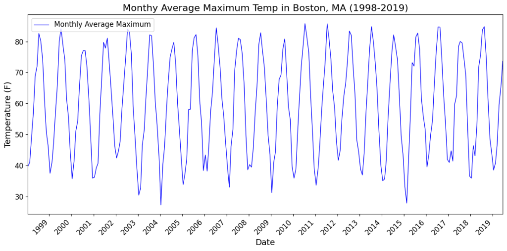
It’s natural to expect January’s maximum from last year to be correlated with the January’s maximum for this year. So we’ll guess the seasonal period to be 12 months. With this assumption, let’s apply a single seasonal difference of 12 months to this time series i.e. we will derive a new time series where each data point is the difference of two data points in the original time series that are 12 periods (12 months) apart. Here’s the seasonally differenced time series:

Next we’ll calculate the PACF of this seasonally differenced time series. Here is the PACF plot:

The PACF plot shows a significant partial autocorrelation at 12, 24, 36, etc. months thereby confirming our guess that the seasonal period is 12 months. Moreover, the fact that these spikes are negative, points to an SMA(1) process. The ‘1’ in SMA(1) corresponds to a period of 12 in the original series. So if you were to construct an Seasonal ARIMA model for this time series, you would set the seasonal component of ARIMA to (0,1,1)12. The middle ‘1’ corresponds to the single seasonal difference we applied, and the next ‘1’ corresponds to the SMA(1) characteristic that we noticed.

There is a lot more to configuring ARIMA and Seasonal ARIMA models. Using the PACF is just one of the tools — albeit one of the front-line tools — for “fixing” the seasonal and non-seasonal orders of this phenomenally powerful class of time series models.

Extending the use of the Partial Correlation Coefficient to linear regression models for cross-sectional data sets

The concept of partial correlation is general enough that it can be easily extended to linear regression models for cross-sectional data. In fact, you’ll see that its application to autoregressive time series models is a special case of its application to linear regression models.

So let’s see how we can compute the partial correlation coefficients of regression variables in a linear model.

Consider the following linear regression model:

To find the partial correlation coefficient of x_k with y, we follow the same 3-step procedure that we followed for time series models:

Step 1

Construct a linear regression model with y as the dependent variable and all variables other than x_k as explanatory variables. Notice below how we’ve left out x_k:

After training this model, we estimate y using the trained model and subtract the estimated y from the observed y to get the vector of residuals ϵ_a.

Step 2

Construct a linear regression model with x_k as the dependent variable and the rest of the variables (except y of course) as regression variables as follows:

After training this model, we estimate x_k using the trained model, and subtract the estimated x_k from the observed x_k to get the vector of residuals ϵb.

STEP 3

Calculate the Pearson’s r between ϵa and ϵb. This is the partial correlation coefficient between x_k and y.

As with the time series data, if the partial correlation coefficient lies within the following confidence interval, we fail to reject the null hypothesis that the coefficient is not statistically significant at a (1 — α)100% confidence level. In that case, we do not include x_k in a linear regression model for estimating y.

Summary

• The partial correlation coefficient measures an explanatory variable’s intrinsic linear influence on the response variable. It does so by eliminating (partialing out) the linear influences of all other candidate explanatory variables in the regression model.
• In a time series settings, the partial autocorrelation coefficient measures the intrinsic linear influence of a time-lagged copy of the response variable on the time-indexed response variable.
• The partial autocorrelation function (PACF) gives you a way to calculate the partial autocorrelations at different time lags.
• While building an AR model for time series data, there are situations when you can use the PACF to precisely identify the lagged copies of the response variable that have a statistically significant influence on the response variable. When the PACF of a suitably differenced time series cuts off sharply after lag k and the lag-1 autocorrelation is positive, you should include the first k time-lags of the dependent variable as explanatory variables in your AR model.
• You may also use the PACF to set the order of a Seasonal Moving Average (SMA) model. Inthe PACF of a seasonally differenced time series, if you detect strong negative correlations at lags s, 2s, 3s, etc. it points to an SMA(1) process.
• Overall, for linear models acting on time series data as well as cross-sectional data, you can use the partial (auto-)correlation coefficient to protect yourself from including irrelevant variables in your regression model, as also to greatly reduce the possibility of accidentally omitting important regression variables from your regression model.

So go ahead, and:

Here’s the link to download the source from GitHub.

Happy modeling!

References and Copyrights

Data sets

The Southern Oscillation Index (SOI) data is downloaded from United States National Weather Service’s Climate Prediction Center’s Weather Indices page. Download link for curated data set.

The Average monthly maximum temperatures data is taken from National Centers for Environmental Information. Download link for the curated data set

Images

All images in this article are copyright Sachin Date under CC-BY-NC-SA, unless a different source and copyright are mentioned underneath the image.

Thanks for reading! If you liked this article, follow me to receive content on statistics and statistical modeling.

How I Learned to Stop Worrying and Love the Partial Autocorrelation Coefficient was originally published in Towards Data Science on Medium, where people are continuing the conversation by highlighting and responding to this story.