Getting started predicting time series data with Facebook Prophet

Getting Started Predicting Time Series Data with Facebook Prophet

This article aims to take away the entry barriers to get started with time series analysis in a hands-on tutorial using Prophet

When getting started with data science, time series analysis is a common thing people would love to try themselves! The general idea here is to learn from historical patterns over time to predict the future. Typical use cases could be weather predictions or sales forecasting. But what does all this have to do with this wise prophet below?!

This article aims to take away the entry barriers to get started with time series analysis in a hands-on tutorial using one of the easiest tools called Facebook Prophet within Google Colab (both are free!). In case you want to get started immediately, feel free to skip the next two chapters where I will give a short background on time series principles and also Facebook Prophet itself. Have fun!

This article is structured into three main sections:

#1 Brief introduction to Time Series Analysis principles
#2 An Introduction to Facebook Prophet
#3 Hands-on tutorial on how to use Prophet in Google Colab (for free)

#1 General Principles of Time Series Analysis

Imagine you are a store manager for consumer products and you want to predict the upcoming product demand to better manage the supply. A reasonable machine learning approach for this scenario is to run some time series analysis which involves understanding, modeling, and making predictions based on sequential data points. [1]

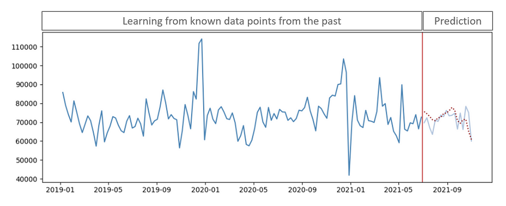
The below graphic illustrates an artificial development of historic product demand (dark-blue line) over time, which can be used to analyze a time series pattern. Our ultimate goal would be to predict (red-dotted line) the actual future demand (light-blue line) as precise as possible:

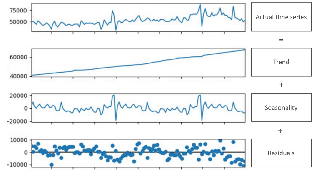
A time series is typically decomposed into three main components:

1. Trend: the long-term movement or general direction in the data.
2. Seasonality: fluctuations or patterns that repeat at regular intervals
3. Residual/error: remainder or leftover variation in the data

The decomposition of a time series into these three components, often referred to as additive or multiplicative decomposition, allows analysts to better understand the underlying structure and patterns. This understanding is essential for selecting appropriate forecasting models and making accurate predictions based on historical data. [2]

#2 What is Facebook Prophet?

Prophet is an open-source tool released by Facebook’s Data Science team that produces time series forecasting data based on an additive model where a non-linear trend fits with seasonality and holiday effects. The design principles allow parameter adjustments without much knowledge of the underlying model which makes the method applicable to teams with less statistical knowledge. [3]

Prophet is particularly well-suited for business forecasting applications, and it has gained popularity due to its ease of use and effectiveness in handling a wide range of time series data. As with every tool, keep in mind that while Prophet is powerful, the choice of forecasting method depends on the specific characteristics of the data and the goals of the analysis. In general, it is not granted that Prophet performs better than other models. However, Prophet comes with some useful features e.g., a reflection of seasonality change pre- and post-COVID or treating lockdowns as one-off holidays.

For a more in-depth introduction by Meta (Facebook) itself, look at the video below on YouTube.

In the following tutorial, we will implement and use Prophet with Python. However, you are more than happy to run your analysis using R as well!

#3 Hands-on tutorial on how to use Prophet

In case you have limited experience with or no access to your coding environment, I recommend making use of Google Colaboratory (“Colab”) which is somewhat like “a free Jupyter notebook environment that requires no setup and runs entirely in the cloud.” While this tutorial claims more about the simplicity and advantages of Colab, there are drawbacks as reduced computing power compared to proper cloud environments. However, I believe Colab might not be a bad service to take the first steps with Prophet.

To set up a basic environment for Time Series Analysis within Colab you can follow these two steps:

1. Open https://colab.research.google.com/ and register for a free account
2. Create a new notebook within Colab
3. Install & use the prophet package:

pip install prophet

from prophet import Prophet

Loading and preparing Data

I uploaded a small dummy dataset representing the monthly amount of passengers for a local bus company (2012–2023). You can find the data here on GitHub.

As the first step, we will load the data using pandas and create two separate datasets: a training subset with the years 2012 to 2022 as well as a test subset with the year 2023. We will train our time series model with the first subset and aim to predict the passenger amount for 2023. With the second subset, we will be able to validate the accuracy later.

import pandas as pd

df_data = pd.read_csv("https://raw.githubusercontent.com/jonasdieckmann/prophet_tutorial/main/passengers.csv")

df_data_train = df_data[df_data["Month"] < "2023-01"]
df_data_test = df_data[df_data["Month"] >= "2023-01"]

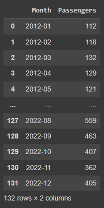
display(df_data_train)

The output for the display command can be seen below. The dataset contains two columns: the indication of the year-month combination as well as a numeric column with the passenger amount in that month. Per default, Prophet is designed to work with daily (or even hourly) data, but we will make sure that the monthly pattern can be used as well.

Decomposing training data

To get a better understanding of the time series components within our dummy data, we will run a quick decomposing. For that, we import the method from statsmodels library and run the decomposing on our dataset. We decided on an additive model and indicated, that one period contains 12 elements (months) in our data. A daily dataset would be period=365.

from statsmodels.tsa.seasonal import seasonal_decompose

decompose = seasonal_decompose(df_data_train.Passengers, model='additive', extrapolate_trend='freq', period=12)

decompose.plot().show()

This short piece of code will give us a visual impression of time series itself, but especially about the trend, the seasonality, and the residuals over time:

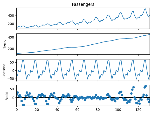
We can now clearly see both, a significantly increasing trend over the past 10 years as well as a recognizable seasonality pattern every year. Following those indications, we would now expect the model to predict some further increasing amount of passengers, following the seasonality peaks in the summer of the future year. But let’s try it out — time to apply some machine learning!

Model fitting with Facebook Prophet

To fit models in Prophet, it is important to have at least a ‘ds’ (datestamp) and ‘y’ (value to be forecasted) column. We should make sure that our columns are renamed the reflect the same.

df_train_prophet = df_data_train

# date variable needs to be named "ds" for prophet
df_train_prophet = df_train_prophet.rename(columns={"Month": "ds"})

# target variable needs to be named "y" for prophet
df_train_prophet = df_train_prophet.rename(columns={"Passengers": "y"})

Now the magic can begin. The process to fit the model is fairly straightforward. However, please have a look at the documentation to get an idea of the large amount of options and parameters we could adjust in this step. To keep things simple, we will fit a simple model without any further adjustments for now — but please keep in mind that real-world data is never perfect: you will definitely need parameter tuning in the future.

model_prophet  = Prophet()
model_prophet.fit(df_train_prophet)

That’s all we have to do to fit the model. Let’s make some predictions!

Making predictions

We have to make predictions on a table that has a ‘ds’ column with the dates you want predictions for. To set up this table, use the make_future_dataframe method, and it will automatically include historical dates. This way, you can see how well the model fits the past data and predicts the future. Since we handle monthly data, we will indicate the frequency with “freq=12″ and ask for a future horizon of 12 months (“periods=12”).

df_future = model_prophet.make_future_dataframe(periods=12, freq='MS')
display(df_future)

This new dataset then contains both, the training period as well as the additional 12 months we want to predict:

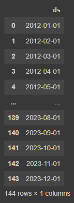
To make predictions, we simply call the predict method from Prophet and provide the future dataset. The prediction output will contain a large dataset with many different columns, but we will focus only on the predicted value yhat as well as the uncertainty intervals yhat_lower and yhat_upper.

forecast_prophet = model_prophet.predict(df_future)
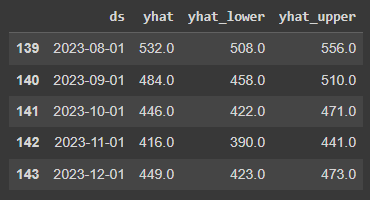
forecast_prophet[['ds', 'yhat', 'yhat_lower', 'yhat_upper']].round().tail()

The table below gives us some idea about how the output is generated and stored. For August 2023, the model predicts a passenger amount of 532 people. The uncertainty interval (which is set by default to 80%) tells us in simple terms that we can expect most likely a passenger amount between 508 and 556 people in that month.

Finally, we want to visualize the output to better understand the predictions and the intervals.

Visualizing results

To plot the results, we can make use of Prophet’s built-in plotting tools. With the plot method, we can display the original time series data alongside the forecasted values.

import matplotlib.pyplot as plt

# plot the time series 
forecast_plot = model_prophet.plot(forecast_prophet)

# add a vertical line at the end of the training period
axes = forecast_plot.gca()
last_training_date = forecast_prophet['ds'].iloc[-12]
axes.axvline(x=last_training_date, color='red', linestyle='--', label='Training End')

# plot true test data for the period after the red line
df_data_test['Month'] = pd.to_datetime(df_data_test['Month'])
plt.plot(df_data_test['Month'], df_data_test['Passengers'],'ro', markersize=3, label='True Test Data')

# show the legend to distinguish between the lines
plt.legend()

Besides the general time series plot, we also added a dotted line to indicate the end of the training period and hence the start of the prediction period. Further, we made use of the true test dataset that we had prepared in the beginning.

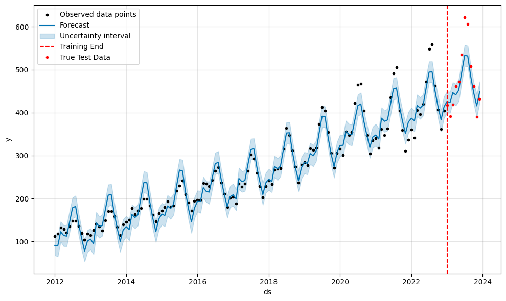
It can be seen that our model isn’t too bad. Most of the true passenger values are actually within the predicted uncertainty intervals. However, the summer months seem to be too pessimistic still, which is a pattern we can see in previous years already. This is a good moment to start exploring the parameters and features we could use with Prophet.

In our example, the seasonality is not a constant additive factor but it grows with the trend over time. Hence, we might consider changing the seasonality_mode from “additive” to “multiplicative” during the model fit. [4]

Our tutorial will conclude here to give some time to explore the large number of possibilities that Prophet offers to us. To review the full code together, I consolidated the snippets in this Python file. Additionally, you could upload this notebook directly to Colab and run it yourself. Let me know how it worked out for you!

Conclusion

Prophet is a powerful tool for predicting future values in time series data, especially when your data has repeating patterns like monthly or yearly cycles. It’s user-friendly and can quickly provide accurate predictions for your specific data. However, it’s essential to be aware of its limitations. If your data doesn’t have a clear pattern or if there are significant changes that the model hasn’t seen before, Prophet may not perform optimally. Understanding these limitations is crucial for using the tool wisely.

The good news is that experimenting with Prophet on your datasets is highly recommended! Every dataset is unique, and tweaking settings and trying different approaches can help you discover what works best for your specific situation. So, dive in, explore, and see how Prophet can enhance your time series forecasting.

Jonas Dieckmann – Medium

I hope you find it useful. Let me know your thoughts! And feel free to connect on LinkedIn https://www.linkedin.com/in/jonas-dieckmann/ and/or to follow me here on medium.

See also some of my other articles:

• How To Use ChatGPT API for Direct Interaction From Colab or Databricks
• How to get started with TensorFlow using Keras API and Google Colab

References

[1] Shumway, Robert H.; Stoffer, David S. (2017): Time Series Analysis and Its Applications. Cham: Springer International Publishing.

[2] Brownlee, Jason (2017): Introduction to Time Series Forecasting With Python

[3] Rafferty, Greg (2021): Forecasting Time Series Data with Facebook Prophet

[4] https://facebook.github.io/prophet/docs/quick_start.html

Getting started predicting time series data with Facebook Prophet was originally published in Towards Data Science on Medium, where people are continuing the conversation by highlighting and responding to this story.