Fine-Tune Smaller Transformer Models: Text Classification

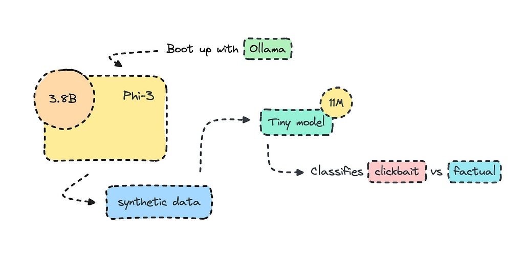
Using Microsoft’s Phi-3 to generate synthetic data

Text classification models aren’t new, but the bar for how quickly they can be built and how well they perform has improved.

The transformer-based model I will fine-tune here is more than 1000 times smaller than GPT-3.5 Turbo. It will perform consistently better for this use case because it will be specifically trained for it.

The idea is to optimize AI workflows where smaller models excel, particularly in handling redundant tasks where larger models are simply overkill.

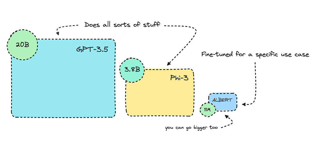
I’ve previously talked about this, where I built a slightly larger keyword extractor for tech-focused content using a sequence-to-sequence transformer model. I also went through the different models and what they excelled at.

For this piece, I’m diving into text classification with transformers, where encoder models do well. I’ll train a pre-trained encoder model with binary classes to identify clickbait versus factual articles. However, you may train it for a different use case.

You’ll find the finished model here.

Most organizations use open-source LLMs such as Mistral and Llama to transform their datasets for training, but what I’ll do here is create the training data altogether using Phi-3 via Ollama.

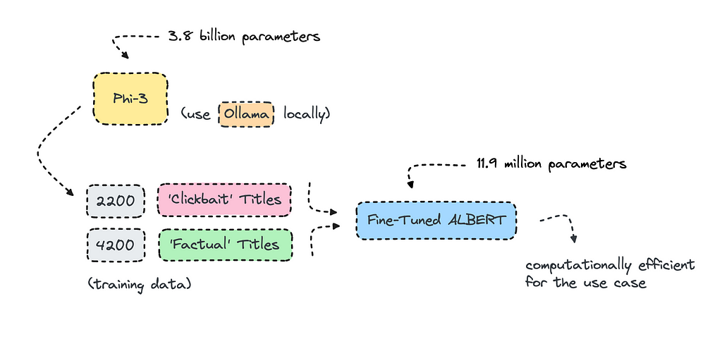
There is always the risk that the model will overfit when using data from a large language model, but in this case, it performed fine, so I’m getting on the artificial data train. However, you will have to be careful and look at the metrics once it is in training.

As for building a text classifier to identify clickbait titles, I think we can agree that some clickbait can be good as it keeps things interesting. I tried the finished model on various titles I made up, and found that having only factual content can be a bit dull.

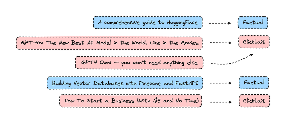
These issues always seem clear-cut, then you dive into them, and they are more nuanced than you considered. The question that popped into my head was, ‘What’s good clickbait content versus bad clickbait content?’ A platform will probably need a bit of both to keep people reading.

I used the new model on all my own content, and none of my titles were identified as clickbait. I’m not sure if that’s something good or not.

If you’re new to transformer encoder models like BERT, this is a good learning experience. If you are not new to building text classification models with transformers, you might find it interesting to see if synthetic data worked well and to look at my performance metrics for this model.

As we all know, it’s easier to use fake data than to access the real thing.

Introduction

I got inspiration for this piece from Fabian Ridder as he was using ChatGPT to identify clickbait and factual articles to train a model using FastText. I thought this case would be great for a smaller transformer model.

The model we’re building will use synthetic data rather than the real thing, though. The process will be quick, as it will only take about an hour or so to generate data with Phi-3 and a few minutes to train it. The model will be very small, with only 11M parameters.

As we’re using binary classes, i.e., clickbait or factual, we will be able to achieve 99% accuracy. The model will have the ability to interpret nuanced texts much better than FastText though.

The cost of training will be zero, and I have already prepared the dataset that we’ll use for this. However, you may generate your own data for another use case.

If you want to dive into training the model, you can skip the introduction where I provide some information on encoder models and the tasks they excel in.

Encoder Models & What They Excel In

While transformers have introduced amazing capabilities in generating text, they have also improved within other NLP tasks, such as text classification and extraction.

The distinction between model architectures is a bit blurry but it’s useful to understand that different transformer models were originally built for different tasks.

A decoder model takes in a smaller input and outputs a larger text. GPT, which introduced impressive text generation back when, is a decoder model. While larger language models offer more nuanced capabilities today, decoders were not built for tasks that involve extraction and labeling. For these tasks, we can use encoder models, which take in more input and provide a condensed output.

Encoders excel at extracting information rather than generating it.

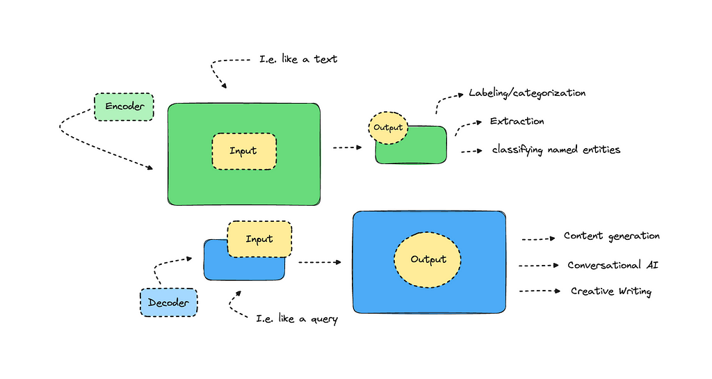
I won’t go into it any more than this, but there should be a lot of information you can scout on the topic, albeit it can be a bit technical.

So, what tasks are popular with encoders? Some examples include sentiment analysis, categorization, named entity recognition, and keyword/topic extraction, among others.

You can try a model that classifies text into twelve different emotions here. You can also look into a model that classifies hate speech as toxic here. Both of these were built with an encoder-only model, in this case, RoBERTa.

There are many base models you can work with; RoBERTa is a newer model that used more data for training and improved on BERT by optimizing its training techniques.

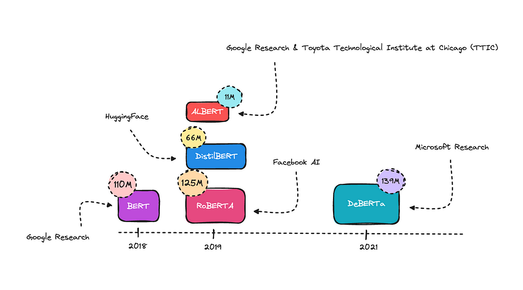
BERT was the first encoder-only transformer model, this one started it all by understanding language context much better than previous models. DistillBERT is a compressed version of BERT.

ALBERT uses some tricks to reduce the number of parameters, making it smaller without significantly losing performance. This is the one I’ll use for this case, as I think it will do well.

DeBERTA is an improved model that better understands word relationships and context. Generally, the bigger models will perform better on complex NLP tasks. However, they can more easily overfit if the training data is not diverse enough.

For this piece, I’m focusing on one task: text classification. So, how hard is it to build a text classification model? It really depends on what you are asking it to do. When working with binary classes, you can achieve a high accuracy score in most cases. However, it also depends on how complex the use case is.

There are certain benchmarks you can look at to understand how BERT has performed with different open-source datasets. I reviewed the paper “How to Fine-Tune BERT for Text Classification?” to look at these benchmarks and graphed their accuracy score with the amount of labels they were trained with below.

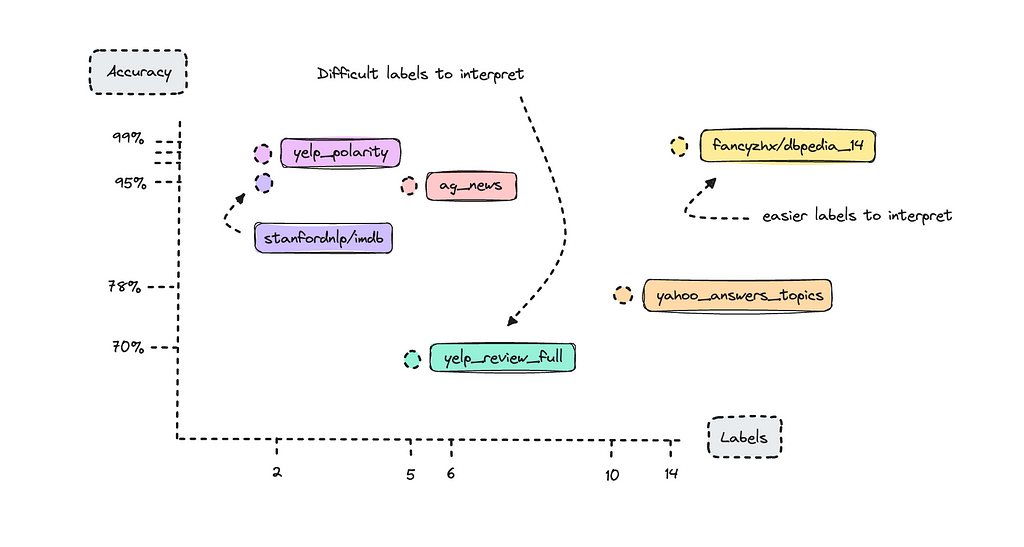
We see datasets with only two labels do quite well. This is what we call binary labels. What might stand out is the DBpedia dataset, which has 14 classes, yet achieved 98% accuracy as a benchmark, whereas the Yelp Review Full dataset, with only 5 classes, achieved only 70%.

Here’s where complexity comes in: Yelp reviews are very difficult to label, especially when rating stars between 1 and 5. Think about how difficult it is for a human to classify someone else’s text into a specific star rating; it really depends on how the person classifies their own reviews.

If you were to build a text classifier with the Yelp reviews dataset, you would find that 1-star and 5-star reviews are labeled correctly most of the time, but the model would struggle with 2, 3, and 4-star reviews. This is because what one person may classify as a 2-star review, the AI model might interpret as a 3-star review.

The DBpedia dataset on the other hand has texts that are easier to interpret for the model.

When we train a model, we can look at the metrics per label rather than as a whole to understand which labels are underperforming. Nevertheless, if you are working with a complex task, don’t feel discouraged if your metrics aren’t perfect.

Always try it afterwards on new data to see if it works well enough on your use case and keep working on the dataset, or switch the underlying model.

The Economics of Smaller Models

I always have a section on the cost of building and running a model. In any project, you’ll have to weigh resources and efficiency to get an outcome.

If you are just trying things out, then a bigger model with an API endpoint makes sense even though it will be computationally inefficient.

I have been running Claude Haiku to do natural language processing for a project now for a month, extracting category, topics and location from texts. This is for demonstration purposes only, but it makes sense when you want to prototype something for an organization.

However, doing zero-shot with these bigger models, will result in a lot of inconsistency, and some texts have to be disregarded altogether. Sometimes the bigger models will output absolute gibberish, but at the same time, it’s cheaper to run them for such a small project.

With your own models you will also have to host them, that’s why we spend so much time trying to make them smaller. You can naturally run them locally, but you’ll probably want to be able to use them for a development project so you’ll need to keep hosting costs in consideration.

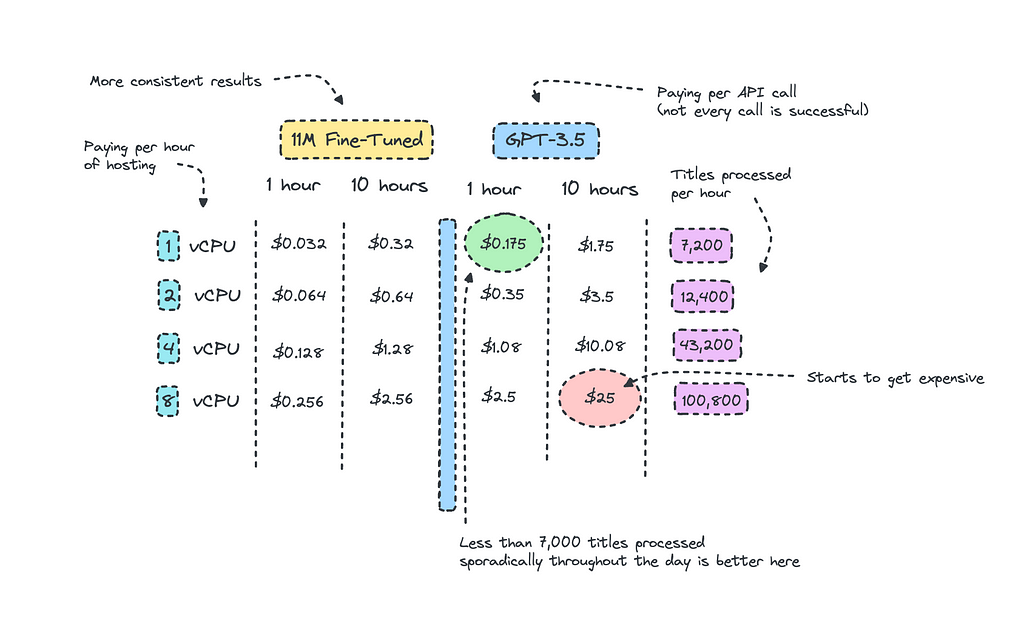
Looking at the picture up top, I have calculated the amount of titles we can process for each instance and compared the same costs for GPT-3.5. I’m aware that it may look a bit messy, but alas it is hard to vizualise.

We can at least deduce that if we are sporadically using GPT-3.5 throughout the day for a small project, it makes sense to use it even though the costs to host the smaller model is quite low.

The breakpoint is when you are consistently processing so much data that surpasses a certain threshold. For this case, this would be when the titles to be processed exceeds 32,000 per day as the cost to keep the instance running 24/7 would equal the same price.

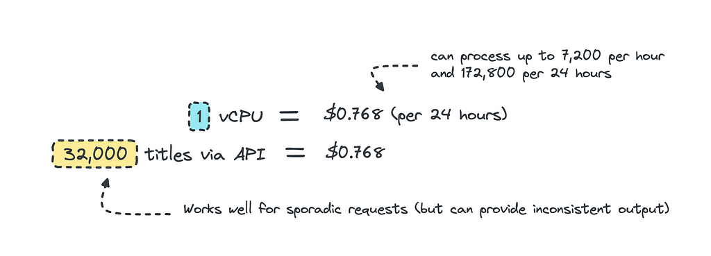
This calculates as if you are keeping the instance running throughout the day, if you are only processing data at certain hours of the day, it makes sense to host and then scale down to zero when it is not in use. Since it’s so small, we can also just containerize it and then host it on ECS or even Lambda for serverless inference.

When using the closed sourced LLMs for zero-shot inference, we would also need to take into account that the model hasn’t been trained for this specific case so we may get inconsistent results. So for redundant tasks where you need consistency, building your own model is a better choice.

It is also worth noting that sometimes you need models that perform on more complex tasks. Here, the cost difference might be steeper for the larger LLMs as you’ll need a better model and a longer prompt template.

Working with Synthetic Data

Transforming data with the use of LLMs isn’t new, if you’re not doing it you should. This is much faster than manually transforming thousands of data points.

I looked at what Orange, the telecom giant, had done via their AI/NLP task force — NEPAL — and they had grabbed data from various places and transformed the raw texts into instruction-like formats using GPT-3.5 and Mixtral to create data that could be used for training.

If you’re keen to read more on this you can look at the session that is provided via Nvidia’s GTC here.

But people are going further than this, using the larger language models to build the entire dataset; this is called synthetic data. It’s a smart way to build smaller specialized models with data that comes from the larger language models but that are cheaper and more efficient to host.

There are concerns at this though, where the quality of synthetic data can be questioned. Relying only on generated data might lead to models that miss nuances or biases inherent in real world data causing it to malfunction when it actually sees it.

However, it is much easier to generate synthetic data than to access the real thing.

Building the Model

I will embark on creating a very simple model here, the model is simply to identify titles as either clickbait or factual. You may build a different text classifier with more labels.

The process is straightforward and I’ll go through the entire process, the cook book we’ll work with is this one.

This tutorial will use this dataset, if you want to build your own dataset be sure to read the first section.

The Dataset

To create a synthetic dataset, we can boot up Ollama locally and run a model we want to use to build the training data. Make sure it is a commercially available model. I chose Phi-3, because it is small and it is very good.

I quite like Javascript, so I used the Ollama JS framework to build a script that could run in the background to produce a CSV file.

This script creates clickbait titles and stores it in a new CSV in your root folder. You need to change the prompt template later to produce an equal amount of titles that are factual.

As I’m using a generative text model, Phi-3, some outputs won’t be usable, but that is to be expected. It will take some time for this to run, so go do something else with your time.

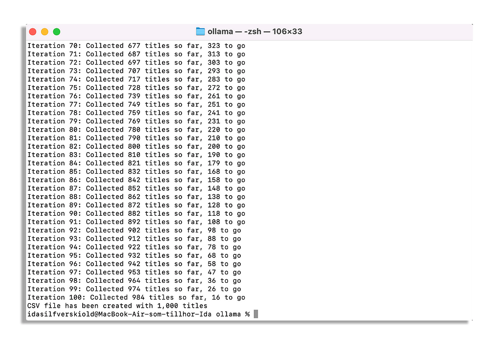
Once you’re finished you can store your finished CSV file with the clickbait and factual tiles in your Google Drive. Remember to set the text and label as fields, where the text is the title and the label is whether it is clickbait or factual.

Since I’ve already prepared the dataset we’ll use, please see this script to upload your custom dataset to HuggingFace.

Looking through the dataset, you’ll see that most clickbait articles that have been generated by Phi-3 has an exclamation mark at the end of it. This is something you want to make sure doesn’t happen, so it’s important to check the work of the LLM generating the data.

Remember that the script I provided you with splits your data into a training, test and validation set. I would recommend to have at least a training and test set for training the model.

If you’ve got your dataset sorted, we can go ahead and fine-tune the model.

Dataset & Model

If you haven’t opened up the cook book, do so here. The first part of this is deciding on your dataset and then your pre-trained model.

from datasets import load_dataset, DatasetDict

dataset = load_dataset("ilsilfverskiold/clickbait_titles_synthetic_data")
dataset

model_name = "albert/albert-base-v2"
your_path = "classify-clickbait"

I wen’t through the different models under the introduction section, where ALBERT and DistillBERT are smaller models and BERT and RoBERTa are larger.

For this case, as it’s not overly complex, I will go for ALBERT. I’m sure BERT can do better, but ALBERT is ten times smaller. RoBERTa is too big and may produce some overfitting with this dataset.

Remember, if you’re working with a different language then look for a base model that has been trained on a corpus from at least a similar language.

If you’re working with nordic languages I can recommend KB/bert-base-swedish-cased that I used to create a model for the IPTC newscodes categories.

Prepare The Dataset

Now we need to do a few things for this to work well.

We first convert our labels to a standardized numerical format that the trainer will understand.

from sklearn.preprocessing import LabelEncoder

label_encoder = LabelEncoder()

label_encoder.fit(dataset['train']['label'])

def encode_labels(example):
    return {'encoded_label': label_encoder.transform([example['label']])[0]}

for split in dataset:
    dataset[split] = dataset[split].map(encode_labels, batched=False)

Then we need to map the numerical representations back to the actual label names. This is so we can get the actual label names rather than the numerical reps when we do inference with the model.

from transformers import AutoConfig

unique_labels = sorted(list(set(dataset['train']['label'])))
id2label = {i: label for i, label in enumerate(unique_labels)}
label2id = {label: i for i, label in enumerate(unique_labels)}

config = AutoConfig.from_pretrained(model_name)
config.id2label = id2label
config.label2id = label2id

# Verify the correct labels
print("ID to Label Mapping:", config.id2label)
print("Label to ID Mapping:", config.label2id)

After this we’re ready to fetch the pre-trained model and it’s tokenizer. We use the config we set up with the labels when we import the model.

from transformers import AlbertForSequenceClassification, AlbertTokenizer

tokenizer = AlbertTokenizer.from_pretrained(model_name)
model = AlbertForSequenceClassification.from_pretrained(model_name, config=config)

If you’re using a different model such as BERT or RoBERTa, you can use AutoTokenizer and AutoModelForSequenceClassification which will automatically select the correct classes for your specified model.

This next function filters for invalid content and then makes sure the text data is properly tokenized and labeled, preparing the dataset for training.

def filter_invalid_content(example):
    return isinstance(example['text'], str)

dataset = dataset.filter(filter_invalid_content, batched=False)

def encode_data(batch):
    tokenized_inputs = tokenizer(batch["text"], padding=True, truncation=True, max_length=256)
    tokenized_inputs["labels"] = batch["encoded_label"]
    return tokenized_inputs

dataset_encoded = dataset.map(encode_data, batched=True)
dataset_encoded

dataset_encoded.set_format(type='torch', columns=['input_ids', 'attention_mask', 'labels'])

We also need to fetch a data collator to handle padding for our inputs.

from transformers import DataCollatorWithPadding

data_collator = DataCollatorWithPadding(tokenizer)

Evaluation Metrics

It’s not required for you to set up any evaluation metrics, such as accuracy, precision, recall or f1. However, you do need at least accuracy to understand how the model is performing.

Accuracy measures the amount of predictions the model got right across all categories. Precision measures how often predictions for a specific category are correct. Recall tells us how well the model can identify all instances within a specific category. The F1 Score is the weighted average of Precision and Recall.

I won’t go into detail on these metrics, but there are many others that write about this. For this case, I’m more interested in how it performs on new real data rather than synthetic data. So, what I look out for are metrics that are too good, indicating that it has overfitted.

We do though set up a function that let us look at the accuracy for each label rather than as an average. This is much more relevant when you have many labels, rather than just two.

from sklearn.preprocessing import LabelEncoder
from sklearn.metrics import accuracy_score, confusion_matrix
import numpy as np

label_encoder = LabelEncoder()
label_encoder.fit(unique_labels)

def per_label_accuracy(y_true, y_pred, labels):
    cm = confusion_matrix(y_true, y_pred, labels=labels)
    correct_predictions = cm.diagonal()
    label_totals = cm.sum(axis=1)
    per_label_acc = np.divide(correct_predictions, label_totals, out=np.zeros_like(correct_predictions, dtype=float), where=label_totals != 0)
    return dict(zip(labels, per_label_acc))

We also set up the general compute metrics function. I am using all of these metrics here because this is general template I have for any text classifier, but you may decide which ones you want.

from sklearn.metrics import accuracy_score, recall_score, precision_score, f1_score

def compute_metrics(pred):
    labels = pred.label_ids
    preds = pred.predictions.argmax(-1)

    decoded_labels = label_encoder.inverse_transform(labels)
    decoded_preds = label_encoder.inverse_transform(preds)

    precision = precision_score(decoded_labels, decoded_preds, average='weighted')
    recall = recall_score(decoded_labels, decoded_preds, average='weighted')
    f1 = f1_score(decoded_labels, decoded_preds, average='weighted')
    acc = accuracy_score(decoded_labels, decoded_preds)

    labels_list = list(label_encoder.classes_)
    per_label_acc = per_label_accuracy(decoded_labels, decoded_preds, labels_list)

    per_label_acc_metrics = {}
    for label, accuracy in per_label_acc.items():
        label_key = f"accuracy_label_{label}"
        per_label_acc_metrics[label_key] = accuracy

    return {
        'accuracy': acc,
        'f1': f1,
        'precision': precision,
        'recall': recall,
        **per_label_acc_metrics
    }

Once you’re decently satisfied, we can move on to setting up the training arguments and the trainer.

Training the Model

Next up we set up our training arguments. Here you can tweak the epochs, batch size and learning rate.

from transformers import Trainer, TrainingArguments

training_args = TrainingArguments(
    output_dir=your_path,
    num_train_epochs=3,
    warmup_steps=500,
    per_device_train_batch_size=16,
    per_device_eval_batch_size=16,
    weight_decay=0.01,
    logging_steps=10,
    evaluation_strategy='steps',
    eval_steps=100,
    learning_rate=2e-5,
    save_steps=1000,
    gradient_accumulation_steps=2
)

I chose to go with a learning rate and epochs based on the paper “How to Fine-Tune BERT for Text Classification?” but decreased the batch size.

Now we can go ahead and set up the trainer, with everything we’ve prepared, and run it.

trainer = Trainer(
    model=model,
    args=training_args,
    train_dataset=dataset_encoded['train'],
    eval_dataset=dataset_encoded['test'],
    compute_metrics=compute_metrics,
    tokenizer=tokenizer,
    data_collator=data_collator,
)

trainer.train()

When in training, you need to look out for overfitting. As both the training and evaluation datasets are synthetic, the typical signs of overfitting might be unclear.

Keep an eye on the accuracy and loss for both the training and evaluation datasets. I.e. very low training and validation loss, along with too stellar evaluation metrics could be a sign of overfitting.

But remember binary classes with less complex tasks usually perform well.

You’ll see my results for one run I made below.

As you can see from the training metrics, they are a bit too good. Validation loss is fluctuating as well. This could be a very bad sign so you have to make sure to test the model on real data once it has finished training.

If you’re training a model with several classes, perhaps even with a skewed dataset, don’t worry if the average evaluation metrics aren’t great. Look at the metrics per label.

Evaluating the Model

Once it’s done training, you can run the final evaluation metrics, save the model and then save the state. This will build the metrics for when you push it to the hub for your model page.

trainer.evaluate()
trainer.save_model(your_path)
trainer.save_state()

Now you can run the HuggingFace pipeline in your notebook to test it.

from transformers import pipeline
pipe = pipeline('text-classification', model=your_path)

example_titles = [
    "grab an example title",
    "grab another example title",
    "and another xample title"
]

for title in example_titles:
    result = pipe(title)
    print(f"Title: {title}")
    print(f"Output: {result[0]['label']}")

Mine did fine on test data, however it missed a few clickbait articles that I personally found to be clickbait. For a production use case, it’s better to build a more diverse dataset (especially with synthetic data) so it can perform well on new real data.

Nevertheless, if you’re not satisfied, then you go back to the dataset, redo it or try with a different model.

If you are wondering, I have indeed gotten stellar results on some runs and less-than-stellar results on other runs with the same data, the same training parameters, and the same seed.

Testing the Model

Before you push the model, you can also test the model against other alternatives.

I asked GPT-3.5 to tell me which titles it thought was clickbait and factual, and it did really well which is to be expected, it is more than 1000x larger than Albert.

We can also compare some titles to what a fine-tuned FastText says versus the fine-tuned transformer encoder model.

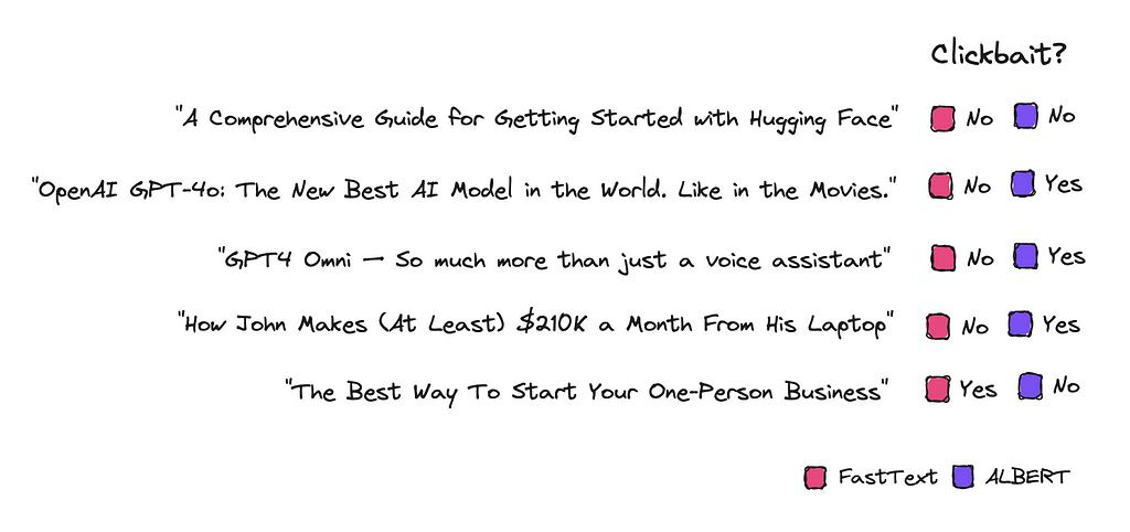
Using FastText is very simple and computationally efficient, but it treats words in isolation and lacks deep contextual understanding.

Therefore, FastText doesn’t capture the context and nuances of language as well as a model that is transformer based.

Push to the Hub

If you’re satisfied with your model, you can push it to the HuggingFace hub to store it there.

You simply login with a write token you can find in your HuggingFace account under Settings.

!huggingface-cli login

And then push it.

tokenizer.push_to_hub("username/classify-clickbait")
trainer.push_to_hub("username/classify-clickbait")

Push the tokenizer just in case, especially if you are working with a version of Albert.

Now you can use it directly from there, mine you’ll find there.

Optimization Techniques

If you want to use a larger model like BERT, you can apply different techniques so you can distill it further after fine-tuning. I didn’t find it that much more successful than just using ALBERT, at least for this case.

BERT on its own though performed much better in general. Although I really like RoBERTa for most cases, it was prone to overfit on this specific dataset either because it was too small, not good enough or too artificial.

For every case you’ll have to estimate how much performance you can sacrifice for efficiency and eventually you learn which models do well in what situation.

Ending Notes

Would the model have performed better if we had used real data? It’s possible, but the accuracy may be lower unless the dataset is meticulously sorted.

This is hard work.

Using synthetic data can get the job done very quickly so you get up a prototype to work with. Synthetic data is much cleaner to work with.

You are also free to work with the larger open source LLMs, so it doesn’t break any rules for people that can’t access high quality data without breaching protocol.

I did not put down time and effort into building this dataset, but in all cases you should make sure you have varied data the model can learn from.

Hopefully this piece was useful and gave you some inspiration and ideas on how to work with the smaller models.

❤

Fine-Tune Smaller Transformer Models: Text Classification was originally published in Towards Data Science on Medium, where people are continuing the conversation by highlighting and responding to this story.