Find Unusual Segments in Your Data with Subgroup Discovery

Patient rule induction method finds 35% better segments than previously reported

Inspired by an in-depth Medium article [1] with a case study on identifying bank customer segments with high churn reduction potential, this story explores a similar challenge through the lens of subgroup discovery methods [2]. Intrigued by the parallels, I applied a subgroup discovery approach to the same dataset and uncovered a segment with a 35% higher churn reduction potential — a significant improvement over what was previously reported. This story will take you through each step of the process, including building the methodology from the ground up. At the end of this journey, you’ll gain:

• A clear understanding of the Patient Rule Induction Method (PRIM), a mature yet powerful subgroup discovery technique.
• The skills to apply PRIM to your datasets and tailor it to your specific needs.

The complete code for PRIM and the experiment is on GitHub [3].

Patient Rule Induction Method

For the experiment, I’ve chosen my favorite subgroup discovery method: PRIM [4]. Despite its long presence in the field, PRIM has a unique mix of properties that make it very versatile:

• Numerical data handling: PRIM easily handles numerical data without the need for binning. Unlike typical methods that discretize variables (e.g., categorizing age into predefined groups such as 45–54 years), PRIM overcomes this limitation. For example, it can identify more nuanced criteria such as age > 37.
• Intelligent categorical data processing: PRIM can discover complex segments within categorical data. It can go beyond simple classifications such as country = Germany to more complex definitions such as country not in {France}.
• Simplicity: While traditional subgroup discovery methods are often burdened with multiple parameters, PRIM is refreshingly simple. It relies primarily on a single, unambiguous peeling parameter: the proportion of points removed from a candidate segment in each iteration.
• Efficiency: Being a heuristic approach, PRIM is remarkably fast. Despite its large search space, segment identification is typically resolved in milliseconds.
• Interactivity and control: PRIM enables interactive analysis. Users can balance segment size against potential impact by examining a series of “nested” segments and selecting the most appropriate one. It also supports incremental segment discovery by removing already segmented data.
• Flexibility: The flexibility of the method extends to the optimization function it is designed to enhance. This function isn’t limited to a single variable. For example, PRIM can identify segments where the correlation between two variables is significantly different from their correlation in the entire data set.

In summary, PRIM’s straightforward logic not only makes it easy to implement, but also allows for customization.

PRIM algorithm

PRIM works through two distinct phases: peeling and pasting. Peeling starts from a segment encompassing the entire dataset and gradually shrinks it while optimizing its quality. Pasting works similarly, but in the opposite direction — it tries to expand the selected candidate segment without quality loss. In our previous experiments [5], we observed that the pasting phase typically contributes minimally to the output quality. Therefore, I will focus on the peeling phase. The underlying logic of the peeling phase is as follows:

1. Initialize:
   - Set the peeling parameter (usually 0.05)
   - Set the initial box (segment) to encompass the entire data space.
   - Define the target quality function (e.g., a potential churn reduction).

2. While the stopping criterion is not met:
   - For each dimension of the data space:
     * Identify a small portion (defined by a peeling parameter) 
       of the data to remove that maximizes quality of remaining data
   - Update the box by removing the identified portion from 
     the current box.
   - Update the dataset by removing the data points that fall outside 
     the new box.

3. End when the stopping criterion is met 
   (e.g., after a certain number of iterations 
   or minimum number of data points remaining).

4. Return the final box and all the preceding boxes as candidate segments.

In this pseudo-code:

• box refers to the current segment of the data.
• The target quality function is typically some statistic of the response variable (mean, median, etc) that we want to maximize or minimize.
• The peeling parameter determines the proportion of data points to be removed in each iteration. It is usually set to a small value, such as 0.05, hence the word “patient” in the method’s name.
• The stopping criterion ensures that enough data points remain for analysis.

Consider simple examples of how PRIM handles numeric and categorical variables:

Numeric variables:
Imagine you have a numeric variable such as age. In each step of the peeling phase, PRIM looks at the range of that variable (say, age from 18 to 80). PRIM then “peels off” a portion of that range from either end, as defined by the peeling parameter. For example, it might remove ages 75 to 80 because doing so improves the target quality function in the remaining data (e.g., increasing the churn reduction potential). The animation below shows PRIM finding an interesting segment (with a high proportion of orange squares) in a 2D numeric dataset.

Categorical nominal variables:
Now consider a categorical nominal variable such as country, with categories such as Germany, France, and Spain. In the peeling phase, PRIM evaluates each category based on how well it improves the target quality function. It then removes the least promising category. For example, if removing “Germany” results in a subset where the target quality function is improved (such as a higher potential churn reduction), then all data points with “Germany” are “peeled”. Note that the peeling parameter has no effect on the processing of categorical data, which can cause undesired effects in some cases, as I will discuss and provide a simple remedy (in section “Better segments via enforced ‘patience’”).

Categorical ordinal variables:
For ordinal variables, disjoint intervals in segment descriptions can sometimes be less intuitive. Consider an education variable with levels such as primary, secondary, vocational, bachelor, and graduate. Finding a rule like education in {primary, bachelor} may not fit well with the ordinal nature of the data because it combines non-adjacent categories. For those looking for a more coherent segmentation, such as education > secondary, that respects the natural order of the variable, using an ordinal encoding can be a useful workaround. For more insight into categorical encoding, you may find my earlier post [6] helpful, as it navigates you to the necessary information.

Experiment: Churn for bank customers

Now everything is ready to start the experiment. Following the Medium article on identifying unique data segments [1], I will apply the PRIM method to the Churn for Bank Customers [7] dataset from Kaggle, available under the CC0: Public Domain license. I will also adopt the target quality function from the article:

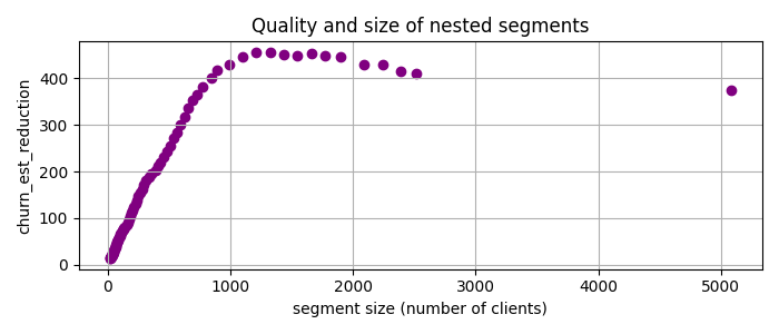
That is, I will look for the segments with many customers where the churn rate is much higher than the baseline, which is the average churn rate in the entire dataset. So I use PRIM, which gives me a set of nested candidate segments, and plot the churn_est_reduction against the number of clients.

The highest quality, churn_est_reduction = 457 is achieved for the 11th candidate segment with the description num_of_products < 2, is_active_member < 1, age > 37. This is quite an improvement over the previously reported maximum churn_est_reduction = 410 in [1]. Comparing the segment descriptions, I suspect that the main reason for this improvement is PRIM’s ability to handle numeric variables.

Better segments via enforced ‘patience’

Something suspicious is going on in the previous plot. By its nature, PRIM is expected to be “patient”, i.e. to reduce the segment size only a little bit at each iteration. However, the second candidate segment is twice as small as the previous one — PRIM has cut off half the data at once. The reason for this is the low cardinality of some features, which is often the case with categorical or indicator variables. For example, is_active_member only takes the values 0 or 1. PRIM can only cut off large chunks of data for such variables, giving them an unfair advantage.

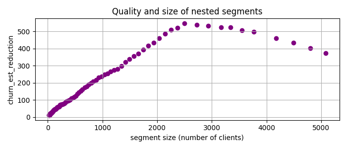
To address this issue, I’ve added an additional parameter called patience to give more weight to smaller cuts. Specifically, for the task at hand, I prioritize cuts by multiplying the churn rate reduction by the segment size raised to the power of patience. This approach helps to fine-tune the selection of segments based on their size, making it more tailored to our analysis needs. Applying PRIM with patience = 2 to the data yields the following candidate segments

Now the best candidate segment is num_of_products < 2, 37 < age < 64 with churn_est_reduction = 548, much better than any previous result!

Finding multiple segments

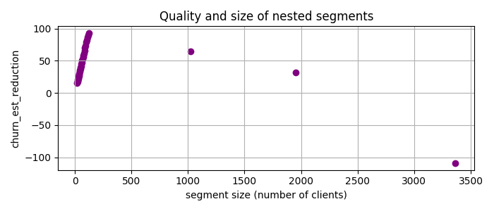
Let us say we have selected the just discovered segment and ask one of two responsible teams to focus on it. Can PRIM find a job for another team, i.e., find another group of clients, not in the first segment, with a high potential churn rate reduction? Yes it can, with so-called “covering” approach [4]. This means that one simply drops the clients belonging to the previously selected segment(s) from the dataset and apply PRIM once again. So I removed data with num_of_products < 2, 37 < age < 64 and applied PRIM to the rest:

Here the best candidate segment is gender != ‘Male’, num_of_products > 2, balance > 0.0 with chirn_est_reduction = 93.

Summary

To wrap things up, I illustrated PRIM’s strong performance on a Customer Churn Dataset for a task to find unusual segments. Points to note:

• PRIM has identified highly insightful segments with 35% higher quality than previously reported.
• I shared the code [3] for practical application and further experimentation. It is very concise and, unlike to other existing implementations [8–9], allows one to easily replace the target quality function tailored to a specific need.
• I endorse PRIM for its robust features, such as effective handling of both numeric and categorical data, flexible segment definition, and fast execution, and recommend it for similar analytical challenges.

References

[1] Figuring out the most unusual segments in data
[2] Atzmueller, Martin. “Subgroup discovery.” Wiley Interdisciplinary Reviews: Data Mining and Knowledge Discovery 5.1 (2015): 35–49.
[3] My code for PRIM and the experiment
[4] Friedman, Jerome H., and Nicholas I. Fisher. “Bump hunting in high-dimensional data.” Statistics and computing 9.2 (1999): 123–143.
[5] Arzamasov, Vadim, and Klemens Böhm. “REDS: rule extraction for discovering scenarios.” Proceedings of the 2021 International Conference on Management of Data. 2021.
[6] Categorical Encoding: Key Insights
[7] Churn for Bank Customers dataset
[8] Patient Rule Induction Method for Python
[9] Patient Rule Induction Method for R

Find Unusual Segments in Your Data with Subgroup Discovery was originally published in Towards Data Science on Medium, where people are continuing the conversation by highlighting and responding to this story.