Feature Engineering for Machine Learning

Enabling the algorithm to work its magic

You must have heard the saying “garbage in, garbage out.” This saying is indeed applicable when training machine learning models. If we train machine learning models using irrelevant data, even the best machine learning algorithms won’t help much. Conversely, using well-engineered meaningful features can achieve superior performance even with a simple machine learning algorithm. So, then, how can we create these meaningful features that will maximize our model’s performance? The answer is feature engineering. Working on feature engineering is especially important when working with traditional machine learning algorithms, such as regressions, decision trees, support vector machines, and others that require numeric inputs. However, creating these numeric inputs is not just about data skills. It’s a process that demands creativity and domain knowledge and has as much art as science.

Broadly speaking, we can divide feature engineering into two components: 1) creating new features and 2) processing these features to make them work optimally with the machine learning algorithm under consideration. In this article, we will discuss these two components of feature engineering for cross-sectional, structured, non-NLP datasets.

New Feature Creation

Raw data gathering can be exhausting, and by the end of this task, we might be too tired to invest more time and energy in creating additional features. But this is where we must resist the temptation of diving straight into model training. I promise you that it will be well worth it! At this junction, we should pause and ask ourselves, “If I were to make the predictions manually based on my domain knowledge, what features would have helped me do a good job?” Asking this question may open up possibilities for crafting new meaningful features that our model might have missed otherwise. Once we have considered what additional features we could benefit from, we can leverage the techniques below to create new features from the raw data.

1. Aggregation

As the name suggests, this technique helps us combine multiple data points to create a more holistic view. We typically apply aggregations on continuous numeric data using standard functions like count, sum, average, minimum, maximum, percentile, standard deviation, and coefficient of variation. Each function can capture different elements of information, and the best function to use depends on the specific use case. Often, we can apply aggregation over a particular time or event window that is meaningful in the context of that problem.

Let’s take an example where we want to predict whether a given credit card transaction is fraudulent. For this use case, we can undoubtedly use transaction-specific features, but alongside those features, we can also benefit from creating aggregated customer-level features like:

1. Count of times the customer has been a fraud victim in the last five years: A customer who has been a fraud victim several times previously may be more likely to be a fraud victim again. Hence, using this aggregated customer-level view can provide proper prediction signals.
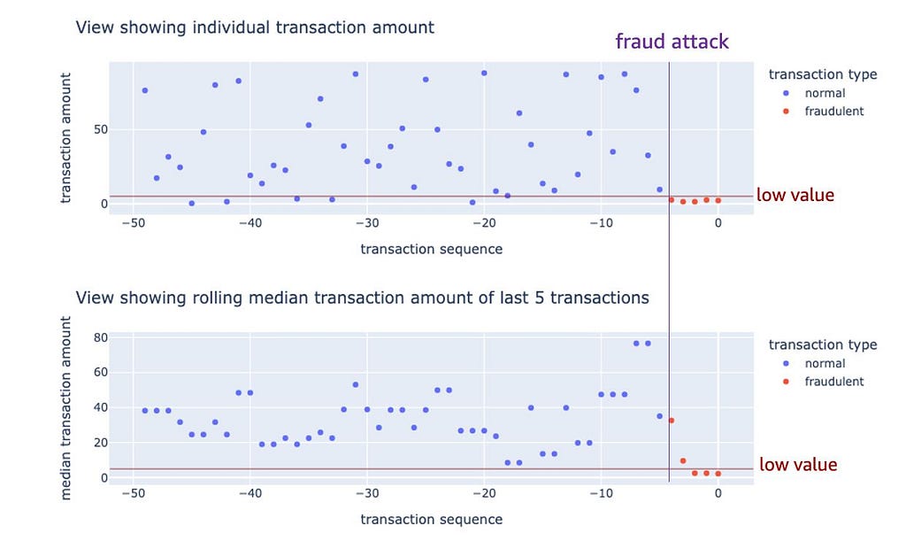
2. Median of last five transaction amounts: Often, when a credit card is compromised, fraudsters may attempt multiple low-value transactions to test the card. Now, a single low-value transaction is very common and may not be a sign of fraud, but if we see many such transactions in short succession, it may indicate a compromised credit card. For a case like, we can consider creating an aggregated feature that takes into account the last few transaction amounts.

2. Differences and Ratios

In many types of problems, change in a set pattern is a valuable signal for prediction or anomaly detection. Differences and ratios are effective techniques for representing changes in numeric features. Just like aggregation, we can also apply these techniques over a meaningful time window in the context of that problem.

Examples:

1. Difference between the percent of new merchant transactions in the last 1 hour and the percent of new merchant transactions in the last 30 days: A high percentage of new merchant transactions in quick succession might indicate fraud risk by itself, but when we see that this behavior has changed as compared to the historical behavior of the customer, it becomes an even more apparent signal.
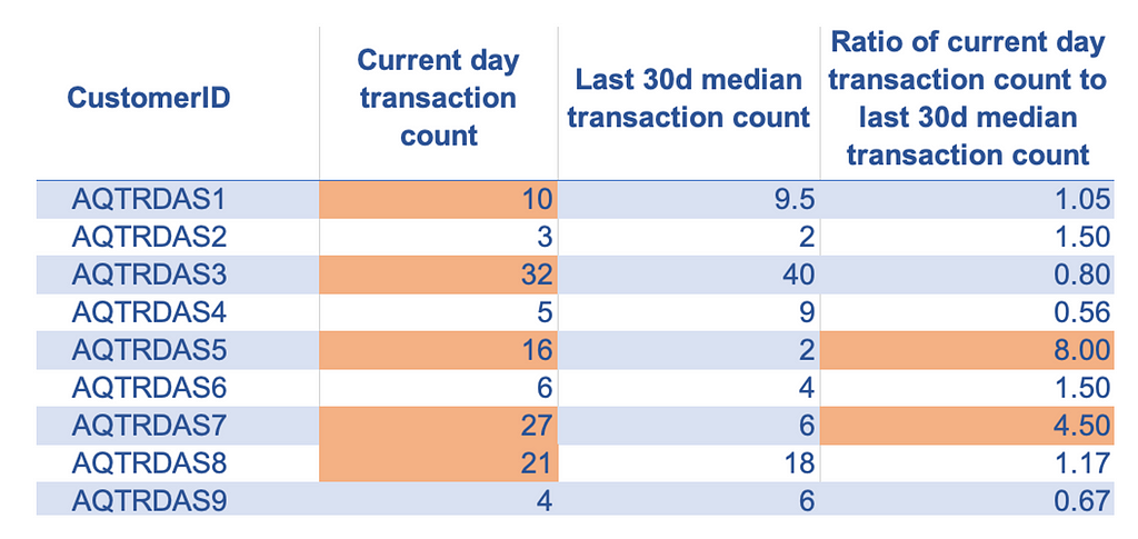
2. Ratio of current-day transaction count to last 30-day median daily transaction count: When a credit card is compromised, it will likely have many transactions in a short time window, which may not conform to past credit card usage. A significantly high ratio of the current-day transaction count to the last 30-day median daily transaction count may indicate fraudulent usage patterns.

3. Age Encoding

We can use the age calculation technique to convert the date or timestamp features to numeric features by taking the difference between two timestamps or dates. We can also use this technique to convert certain non-numeric features into meaningful numeric features if the tenure associated with the feature values can be a valuable signal for prediction.

Examples:

1. Days since the credit card was last used: A sudden transaction on a credit card that has been dormant for a long time may be associated with a high risk of fraud. We can calculate this feature by taking the time difference between the date since the credit card was last used and the current transaction date.
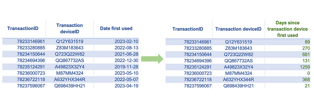
2. Days since the customer’s device was first used: If we see a transaction coming from a new device, it is likely to be riskier than a transaction made from a device the customer has used for a longer time. We can create a feature that indicates the age of the device as the difference between the date since the customer first used this device and the current transaction date.

4. Indicator Encoding

Indicator or Boolean features have binary values {1, 0} or {True, False}. Indicator features are very common and are used to represent various types of binary information. In some cases, we may already have such binary features in numeric form, while in other instances, they may have non-numeric values. To use the non-numeric binary features for model training, all we have to do is map them to numeric values.

Looking beyond these common occurrences and uses of indicator features, we can leverage indicator encoding as a tool to represent a comparison between non-numeric data points. This attribute makes it particularly powerful as it creates a way for us to measure the changes in non-numeric features.

Examples:

1. Failed verification during recent login event: A recent failed login event may be associated with a higher risk of fraudulent transactions. In this case, the raw data may have Yes or No values for this feature; all we have to do here is map these values to 1 or 0.
2. Change in the country location from the last transaction: A change in country location may indicate a compromised credit card. Here, creating an indicator feature representing a change in the non-numeric feature ‘country location’ will capture this country change information.

5. One-Hot Encoding

This technique can be applied if our feature data is in categorical form, either numeric or non-numeric. The numeric-categorical form refers to numeric data containing non-continuous or non-measurement data, such as geographical region codes, store IDs, and other such types of data. One hot encoding technique can convert such features into a set of indicator features that we can use in training machine learning models. Applying one hot encoding on a categorical feature will create one new binary feature for every category in that categorical variable. Since the number of new features increases as the number of categories increases, this technique is suitable for features with a low number of categories, especially if we have a smaller dataset. One of the standard rules of thumb suggests applying this technique if we have at least ten records per category.

Examples:

1. Transaction purchase category: Certain types of purchase categories may be associated with a higher risk of fraud. Since the purchase category names are text data, we can apply the one-hot encoding technique to convert this feature into a set of numeric indicator features. If there are ten different purchase category names, one-hot encoding will create ten new indicator features, one for each purchase category name.
2. Device type: An online transaction could be made through several different types of devices, such as an iPhone, Android phone, Windows PC, and Mac. Some of these devices are more susceptible to malware or easily accessible to fraudsters and, therefore, may be associated with a higher risk of fraud. To include device type information in numeric form, we may apply one-hot encoding to the device type, which will create a new indicator feature for each device type.

6. Target Encoding

This technique is applied to the same type of features that we would apply the one-hot encoding to but has some advantages and disadvantages over one-hot encoding. When the number of categories is high (high cardinality), using one-hot encoding will undesirably increase the number of features, which may lead to model overfitting. Target encoding can be an effective technique in such cases, provided we are working on a supervised learning problem. It is a technique that maps each category value to the expected value of the target for that category. If working with a regression problem with a continuous target, this calculation maps the category to the mean target value for that category. In the case of a classification problem with a binary target, target encoding will map the category to the positive event probability of that category. Unlike one-hot encoding, this technique has the advantage of not increasing the number of features. A downside of this technique is that it can only be applied to supervised learning problems. Applying this technique may also make the model susceptible to overfitting, particularly if the number of observations in some categories is low.

Examples:

1. Merchant name: Transactions placed against certain merchants could indicate fraudulent activity. There could be thousands of such merchants, each with a different risk of fraudulent transactions. Applying one-hot encoding to a feature containing merchant names may introduce thousands of new features, which is undesirable. In such cases, target encoding can help capture the merchant’s fraud risk information without increasing the number of features.
2. Transaction zip code: Just like merchants, transactions made in different zip codes may represent different fraud risk levels. Although zip codes have numeric values, they are not continuous measurement variables and should not be used in the model as is. Instead, we can incorporate the fraud risk information associated with each zip code by applying a technique like target encoding.

Once we have created the new features from the raw data, the next step is to process them for optimal model performance. We accomplish this though feature processing as discussed in the next section.

Feature Processing

Feature processing refers to series of data processing steps that ensure that the machine learning models fit the data as intended. While some of these processing steps are required when using certain machine learning algorithms, others ensure that we strike a good working chemistry between the features and the machine learning algorithm under consideration. In this section, let’s discuss some common feature processing steps and why we need them.

1. Outlier Treatment

Several machine learning algorithms, especially parametric ones such as regression models, are severely impacted by outliers. These machine learning algorithms attempt to accommodate outliers, severely affecting the model parameters and compromising overall performance. To treat the outliers, we must first identify them. We can detect outliers for a specific feature by applying certain rules of thumb, such as having an absolute value greater than the mean plus three standard deviations or a value outside the nearest whisker value (nearest quartile value plus 1.5 times the interquartile range value). Once we have identified the outliers in a specific feature, we can use some of the techniques below to treat outliers:

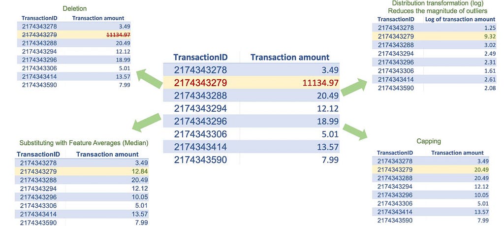
1. Deletion: we can delete the observations with at least one outlier value. However, if our data has too many outlier values across different features, we may lose many observations.
2. Substituting: We can substitute outlier values with averages, such as the mean, median, and mode, of a given feature.
3. Feature transformation or standardization: we can use log transformation or feature standardization (as described in scaling) to reduce the magnitude of the outliers.
4. Capping and flooring: we can replace the outliers beyond a certain value with that value, for example, replacing all values above the 99th percentile with the 99th percentile value and replacing all values below the 1st percentile with the 1st percentile value.

Note that there are techniques to detect observations that are multivariate outliers (outliers with respect to multiple features), but they are more complex and generally do not add much value in terms of machine learning model training. Also note that outliers are not a concern when working with most non-parametric machine learning models like support vector machines and tree-based algorithms like decision trees, random forests, and XGBoost.

2. Missing Values Treatment

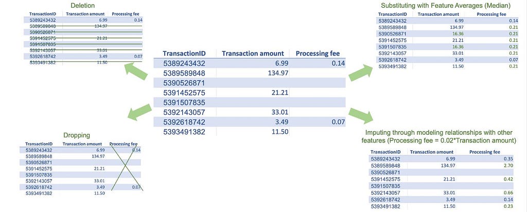
Missing data is very common in real-world datasets. Most traditional machine learning algorithms, except a few like XGBoost, don’t allow missing values in training datasets. Thus, fixing missing values is one of the routine tasks in machine learning modeling. There are several techniques to treat missing values; however, before implementing any technique, it is important to understand the cause of the missing data or, at the very least, know if the data is missing at random. If the data is not missing at random, meaning certain subgroups are more likely to have missing data, imputing values for those might be difficult, especially if there is little to no data available. If the data is missing at random, we can use some of the common treatment techniques described below. They all have pros and cons, and it’s up to us to decide what method best suits our use case.

1. Deletion: We can delete the observations with at least one missing feature value. However, if our data has too many missing values across different features, we may end up losing many observations.
2. Dropping: If a feature has a large number of missing values, we can choose to drop it.
3. Substituting with averages: We can use averages like the mean, median, and mode of a given feature to substitute for the missing values. This method is simple to implement, but it may not provide good estimates for all types of observations. For example, a high fraud risk transaction may have a different average transaction amount than a low fraud risk transaction amount, and using an overall average for a missing high fraud risk transaction amount may not be a good substitution.
4. Maximum likelihood, multiple imputations, K nearest neighbors: These are more complex methods that consider the relationship with other features in the dataset and could provide more accurate estimates than overall averages. However, implementing these methods will require additional modeling or algorithm implementation.

3. Scaling

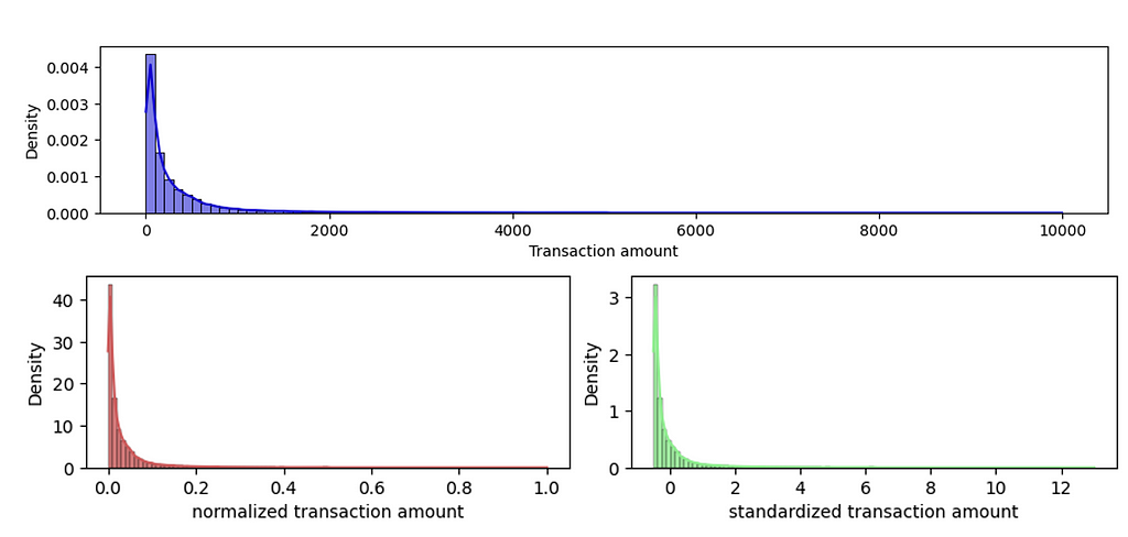
Often, features that we use in machine learning models have different ranges. If we use them without scaling, the features with large absolute values will dominate the prediction outcome. Instead, to give each feature a fair opportunity to contribute to the prediction outcome, we must bring all features on the same scale. The two most common scaling techniques are:

1. Normalization: This scaling technique restricts the feature values between 0 and 1. To apply normalization, we subtract the minimum feature value and divide it by the range (difference between min and max) of that feature. Normalization may not be a good technique if some of our features have a sharp skew or have a few extreme outliers.
2. Standardization: This technique transforms the feature data distribution to the standard normal distribution. We can implement this technique by subtracting the mean and dividing it by the standard deviation. This technique is generally preferred if the feature has a sharp skew or a few extreme outliers.

Note that tree-based algorithms like decision trees, random forest, XGBoost, and others can work with unscaled data and do not need scaling when using these algorithms.

4. Dimensionality Reduction

Today, we have enormous data, and we can build a vast collection of features to train our models. For most algorithms, having more features is good since it provides more options to improve the model performance. However, this is not true for all algorithms. Algorithms based on distance metrics suffer from the curse of dimensionality — as the number of features increases substantially, the distance value between the two observations becomes meaningless. Thus, to use algorithms that rely on distance metrics, we should ensure that we are not using a large number of features. If our dataset has a large number of features and if we don’t know which ones to keep and which to discard, we can use techniques like Principal component analysis (PCA). PCA transforms the set of old features into a set of new features. It creates new features such that the one with the highest eigenvalues captures most of the information from the old features. We can then keep only the top few new features and discard the remaining ones.

Other statistical techniques, such as association analysis and feature selection algorithms, can be used in supervised learning problems to reduce the number of features. However, they generally do not capture the same level of information that PCA does with the same number of features.

5. Transforming to Normal Distribution

This step is an exception because it only applies to the target and not to the features. Also, most machine learning algorithms don’t have any restrictions on the target’s distribution, but certain ones like linear regression, require that the target to be distributed normally. Linear regression assumes that the error values are symmetric and concentrated around zero for all the data points (just like the shape of the normal distribution), and a normally distributed target variable ensures that this assumption is met. We can understand our target’s distribution by plotting a histogram. Statistical tests like the Shapiro-Wilk test tell us about the normality by testing this hypothesis. In case our target is not normally distributed, we can try out various transformations such as log transform, square transform, square root transform, and others to check which transforms make the target distribution normal. There is also a Box-Cox transformation that tries out multiple parameter values, and we can choose the one that best transforms our target’s distribution to normal.

Note: While we can implement the feature processing steps in features in any order, we must thoroughly consider the sequence of their application. For example, missing value treatment using value mean substitution can be implemented before or after outlier detection. However, the mean value used for substitution may differ depending on whether we treat the missing values before or after the outlier treatment. The feature processing sequence outlined in this article treats the issues in the order of the impact they can have on the successive processing steps. Thus, following this sequence should generally be effective for addressing most problems.

Conclusion

As mentioned in the introduction, feature engineering is a dimension of machine learning that allows us to control the model’s performance to an exceptional degree. To exploit feature engineering to its potential, we learned various techniques in this article to create new features and process them to work optimally with machine learning models. No matter what feature engineering principles and techniques from this article you choose to use, the important message here is to understand that machine learning is not just about asking the algorithm to figure out the patterns. It is about us enabling the algorithm to do its job effectively by providing the kind of data it needs.

Unless otherwise noted, all images are by the author.

Feature Engineering for Machine Learning was originally published in Towards Data Science on Medium, where people are continuing the conversation by highlighting and responding to this story.