Dissolving map boundaries in QGIS and Python

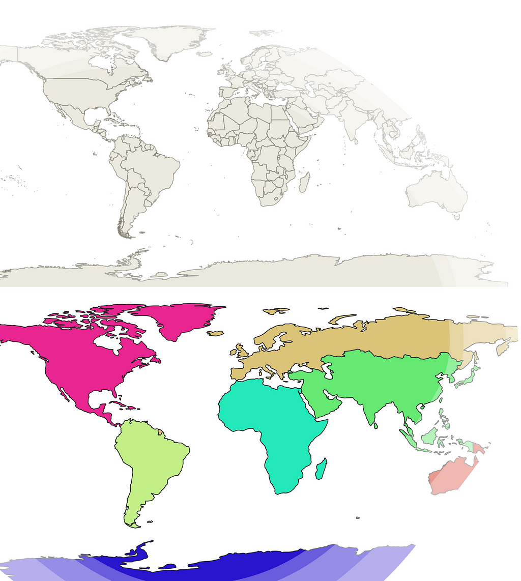
This post describes some interesting processes for transforming the map boundaries in vector datasets using QGIS and geopandas in Python.

Recently, for one of my projects, I had to define the composition of countries in a region, make the region distinct, and highlight it on the map of a continent. Let’s take an example of the South Asia region in Asia. The South Asia region is comprised of eight countries: Afghanistan, Bangladesh, Bhutan, India, Maldives, Nepal, Pakistan and Sri Lanka. From the map of Asia, I wanted to clip off the South Asia region and highlight it distinctly in the continental map. Furthermore, I wanted to go one step ahead and dissolve the boundaries of the countries in the region so that the region could be demonstrated as a single unit.

I was able to achieve this using both Quantum-GIS (QGIS) and geopandas package in Python. In this process, I utilized the clipping feature which I was already familiar with, and I learned about the dissolve feature which I found very fascinating. In this post, I am going to share my learning about these features and how I achieved my objectives. Let’s get started.

1. QGIS

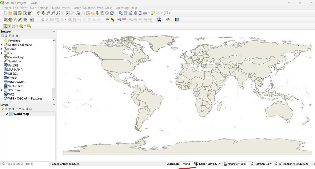
In an empty QGIS project, by typing world in the coordinate space in the bottom of the page, I could call an in-built map of the world with administrative boundaries of all the countries as shown below.

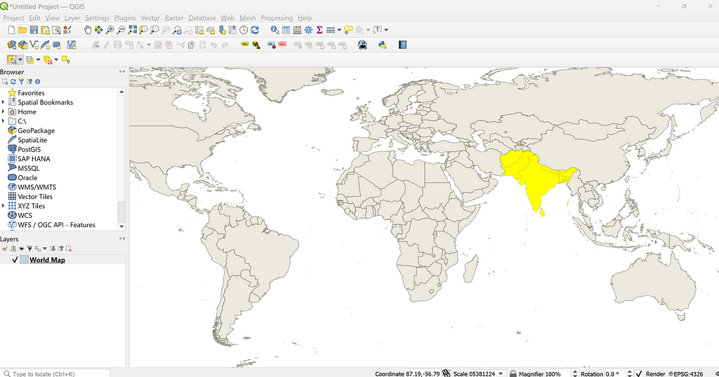
Next, by using the select feature, I selected the 8 countries of South Asia as highlighted in the map below. QGIS offers the option to select countries by hand, by polygon, by radius, and by individually selecting or deselecting countries with a mouse click.

Clipping in QGIS

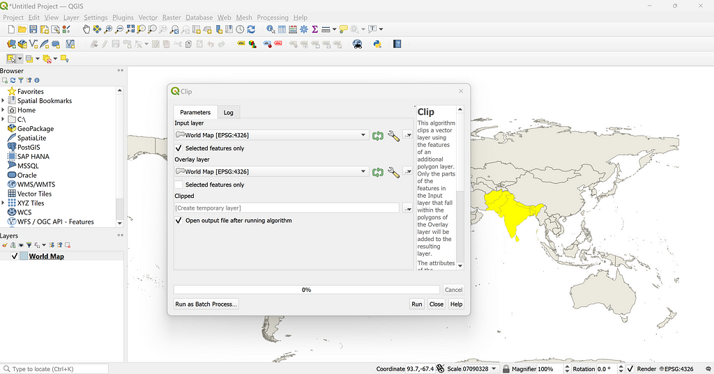
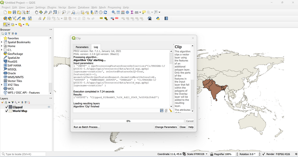
Clipping these countries off of the world map is straightforward in QGIS. One needs to go to Vector in the menu-> Select Geoprocessing tools -> Select Clip. In the options, I ticked on the check box for the Selected features only in the Input layer and ran the process.

The clipping action was completed in 7.24 seconds alone and I got a new layer called “Clipped”. This is depicted by the brown color in the screenshot below. By going to Properties of the layer, one can use different coloring options in QGIS in the Symbology option.

Dissolving boundaries in QGIS

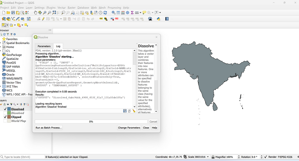
Next, I wanted to dissolve the boundaries between countries in South Asia. For this, I selected all the countries in South Asia. I went to the Vector Menu -> Select Geoprocessing Tools ->Dissolve. Similar to the previous step, I selected “Selected featured only” in the input layer and ran the algorithm which took just 0.08 seconds. A new layer called “Dissolved” was created where the administrative boundaries between countries were dissolved and appeared as a single unit as shown below:

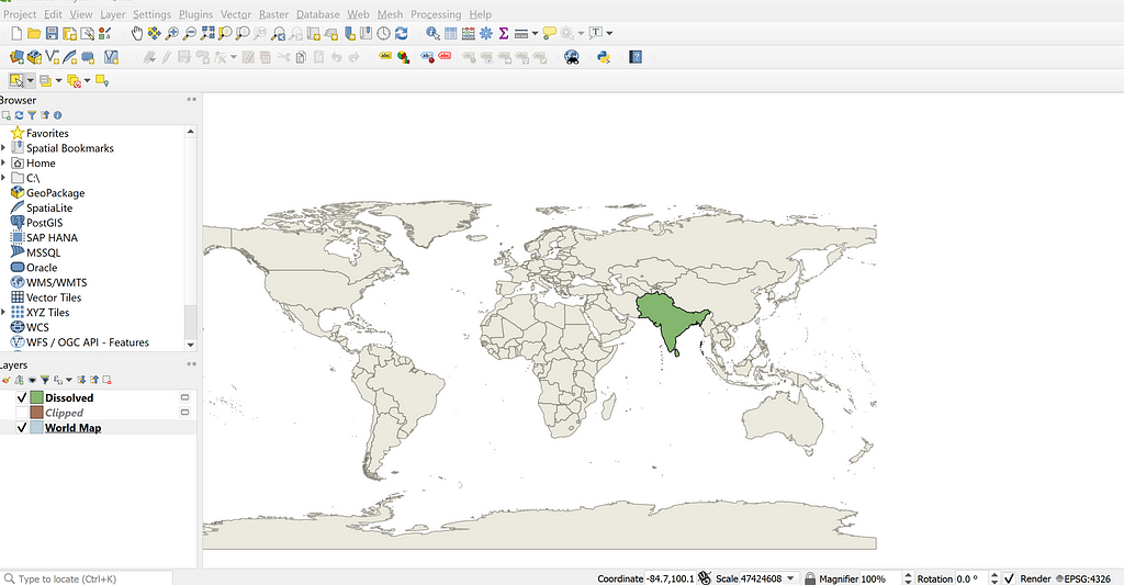
Visualizing both the world layer and Dissolved layer at the same time looks as shown below:

2. Geopandas

In this section, I am going to demonstrate how I could the same objective in Python using the geopandas package.

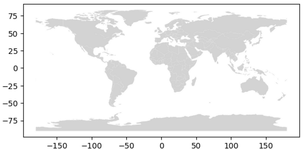
In the first step, I read the in-built dataset of the world map within the geopandas package. It contains the vector data of the world with the administative boundaries of all counntries. This is obtained from the Natural Earth dataset, which is free to use.

import pandas as pd
import geopandas as gpd
import matplotlib.pyplot as plt
import numpy as np

world = gpd.read_file(gpd.datasets.get_path('naturalearth_lowres'))
world.plot(color = "lightgrey")

Clipping with geopandas

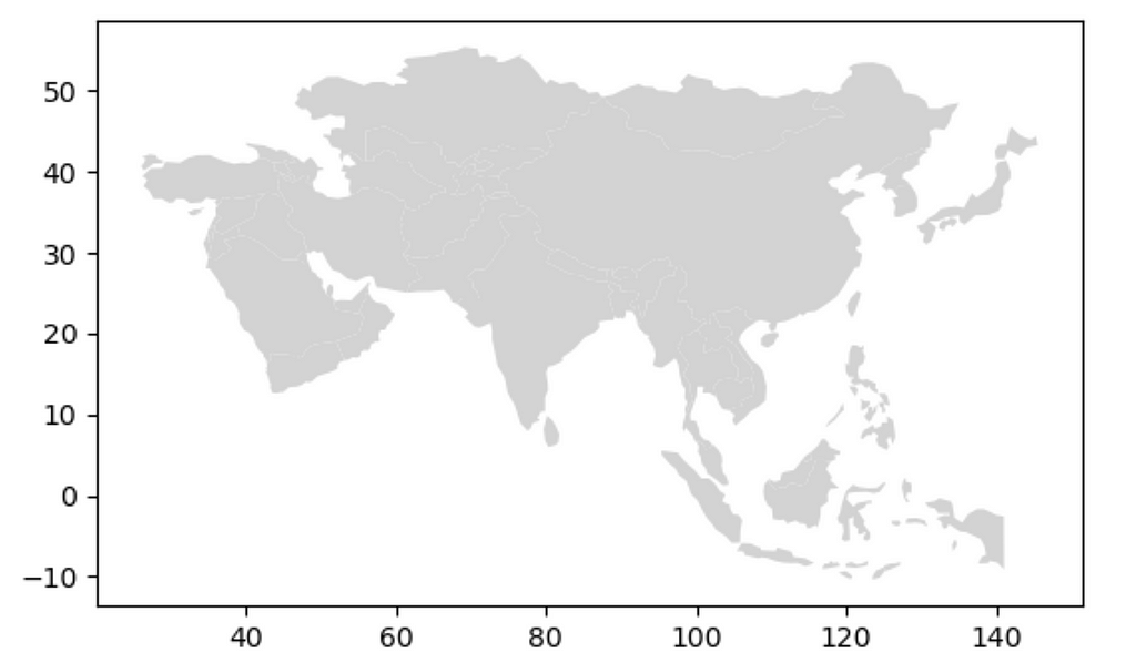
In my very first post, I demonstrated how it is possible to clip off a custom Polygon geometry as a mask from the original geopandas dataframe or layer. However, for simplicity, I just used the filter options to obtain the required layers for Asia and South Asia.

asia = world[world.continent == "Asia"]
asia.plot(color = "lightgrey")

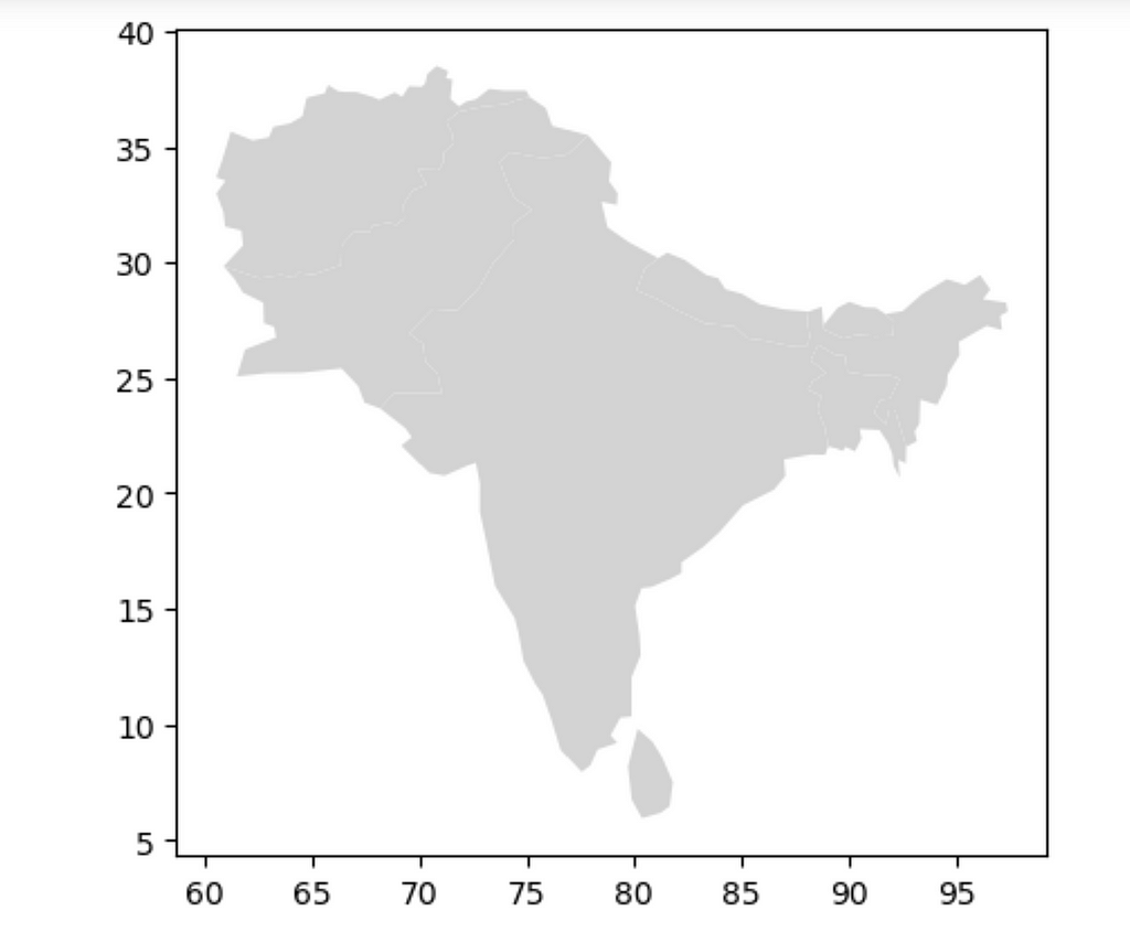
To filter the South Asia region, I used a list containing the name of each country as a reference.

south_asia_countries = ["Afghanistan", "Bangladesh", "Bhutan", "India",
                       "Maldives", "Nepal", "Pakistan", "Sri Lanka"]

south_asia = asia[asia.name.isin(south_asia_countries)]

south_asia.plot()

Dissolve boundaries between countries in South Asia using geopandas

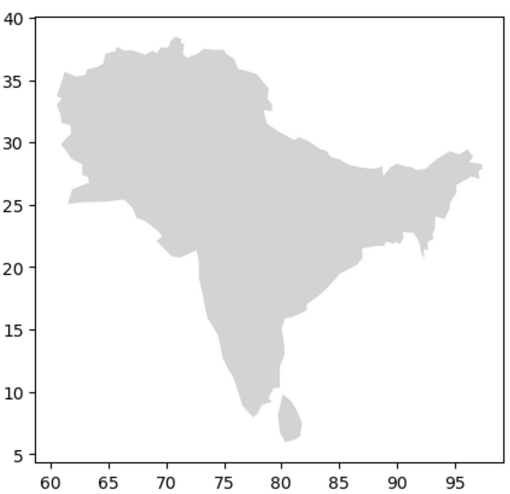
To dissolve the boundaries between countries in South Asia, I used the dissolve feature in geopandas. I passed None as an argument, and specified parameters to apply certain aggregate functions, in which the population and GDP in the resulting dissolved dataframe would sum up the population and GDP in all countries in South Asia. I am yet to figure out how the aggregate function can also be applied in QGIS.

south_asia_dissolved = south_asia.dissolve(by = None,
                                          aggfunc = {"pop_est":"sum",
                                                    "gdp_md_est":"sum"})
south_asia_dissolved.plot(color = "lightgrey"

Dissolving boundaries between countries within a continent in the world

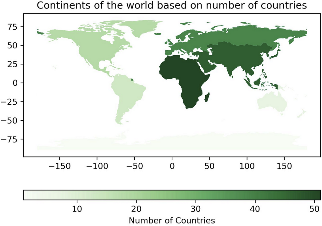
Using the same procedure as above, I wanted to dissolve the boundaries between countries within a continent and show different continents distinct from each other in a world map based on the number of countries in each continent.

For this purpose, first I added a new column called num_countries in the world geodataframe containing 1 as a value. Then I dissolved the world map using the continent column as a reference.

world["num_countries"] = 1

continents_dissolved = world.dissolve(by = "continent", 
                      aggfunc = {"pop_est":"sum",
                                 "gdp_md_est":"sum",
                               "num_countries":"count"}).reset_index()

continents_dissolved

I used the aggregate function to sum up the population and GDP in all countries in the continent and count the number of countries in each continent. The resulting geodataframe continents_dissolved look as shown:

We see that Asia has the largest population and GDP of all continents. Similarly, we see that Africa has the most countries (51) followed by Asia (47), Europe (39), North America (18), South America (13), and Oceania (7). Antarctica and Seven seas (open ocean) are also regarded as continents in this dataset.

Finally, I wanted to plot the world map highlighting the number of countries in each continent with the help of a color map. I achieved this using the following code:

map = continents_dissolved.plot(column = "num_countries",
                         cmap = "Greens")

# Get the current axes
ax = plt.gca()

# Add a horizontal colorbar
cbar = plt.colorbar(map.get_children()[0],
                    ax=ax, 
                    orientation='horizontal',
                   aspect = 30   #control the width of color bar. higher value= lower width.
                   )

# Set a label for the colorbar
cbar.set_label('Number of Countries')

plt.title("Continents of the world based on number of countries")

plt.savefig("Continents dissolved.jpeg",
            bbox_inches = "tight",
           dpi = 300)

# Show the plot
plt.show()

The resulting map appears as shown below:

Conclusion

In this post, I described ways to dissolve map boundaries using QGIS and geopandas in Python. In the process, I also explained the clipping process and the possibility of using aggregate function while dissolving the map boundaries in geopandas. These processes could be very useful for the manipulation, processing, and transformation of geographical maps in the form of vector datasets. The code and the QGIS project file for this post are available in this GitHub repository. Thank you for reading!

Dissolving map boundaries in QGIS and Python was originally published in Towards Data Science on Medium, where people are continuing the conversation by highlighting and responding to this story.