Diffusion Model from Scratch in Pytorch

Implementation of Denoising Diffusion Probabilistic Models (DDPM)

Introduction

A diffusion model in general terms is a type of generative deep learning model that creates data from a learned denoising process. There are many variations of diffusion models with the most popular ones usually being text conditional models that can generate a certain image based on a prompt. Some diffusion models (Control-Net) can even blend images with certain artistic styles. Here is an example below here:

If you don’t know what’s so special about the image, try moving farther away from the screen or squinting your eyes to see the secret hidden in the image.

There are many different applications and types of diffusion models, but in this tutorial we are going to build the foundational unconditional diffusion model, DDPM (Denoising Diffusion Probabilistic Models) [1]. We will start by looking into how the algorithm works intuitively under the hood, and then we will build it from scratch in PyTorch. Also, this tutorial will focus primarily on the intuitive idea behind the algorithm and the specific implementation details. For the mathematical derivations and background, this book [2] is a great reference.

Last Notes: This implementation was built for workflows that contain a single GPU with CUDA compatibility. In addition, the complete code repository can be found here https://github.com/nickd16/Diffusion-Models-from-Scratch

How it Works -> The Forward and Reverse Process

The diffusion process includes a forward and a reverse process. The forward process is a predetermined Markov chain based on a noise schedule. The noise schedule is a set of variances B1, B2, … BT that govern the conditional normal distributions that make up the Markov chain.

This formula is the mathematical representation of the forward process, but intuitively we can understand it as a sequence where we gradually map our data examples X to pure noise. Our first term in the forward process is just our initial data example. At an intermediate time step t, we have a noised version of X, and at our final time step T, we arrive at pure noise that is approximately governed by a standard normal distribution. When we build a diffusion model, we choose our noise schedule. In DDPM for example, our noise schedule features 1000 time steps of linearly increasing variances starting at 1e-4 to 0.02. It is also important to note that our forward process is static, meaning we choose our noise schedule as a hyperparameter to our diffusion model and we do not train the forward process as it is already defined explicitly.

The final key detail we have to know about the forward process is that because the distributions are normal, we can mathematically derive a distribution known as the “Diffusion Kernel” which is the distribution of any intermediate value in our forward process given our initial data point. This allows us to bypass all of the intermediate steps of iteratively adding t-1 levels of noise in the forward process to get an image with t noise which will come in handy later when we train our model. This is mathematically represented as:

where alpha at time t is defined as the cumulative product (1-B) from our initial time step to our current time step.

The reverse process is the key to a diffusion model. The reverse process is essentially the undoing of the forward process by gradually removing amounts of noise from a pure noisy image to generate new images. We do this by starting at purely noised data, and for each time step t we subtract the amount of noise that would have theoretically been added by the forward process for that time step. We keep removing noise until eventually we have something that resembles our original data distribution. The bulk of our work is training a model to carefully approximate the forward process in order to estimate a reverse process that can generate new samples.

The Algorithm and Training Objective

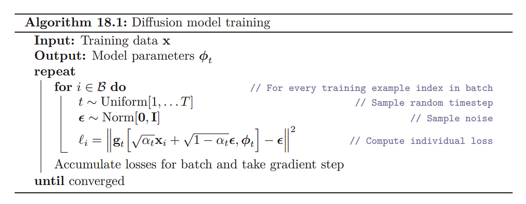
To train such a model to estimate the reverse diffusion process, we can follow the algorithm in the image defined below:

1. Take a randomly sampled data point from our training dataset
2. Select a random timestep on our noise (variance) schedule
3. Add the noise from that time step to our data, simulating the forward diffusion process through the “diffusion kernel”
4. Pass our defused image into our model to predict the noise we added
5. Compute the mean squared error between the predicted noise and the actual noise and optimize our model’s parameters through that objective function
6. And repeat!

Mathematically, the exact formula in the algorithm might look a little strange at first without seeing the full derivation, but intuitively its a reparameterization of the diffusion kernel based on the alpha values of our noise schedule and its simply the squared difference of predicted noise and the actual noise we added to an image.

If our model can successfully predict the amount of noise based on a specific time step of our forward process, we can iteratively start from noise at time step T and gradually remove noise based on each time step until we recover data that resembles a generated sample from our original data distribution.

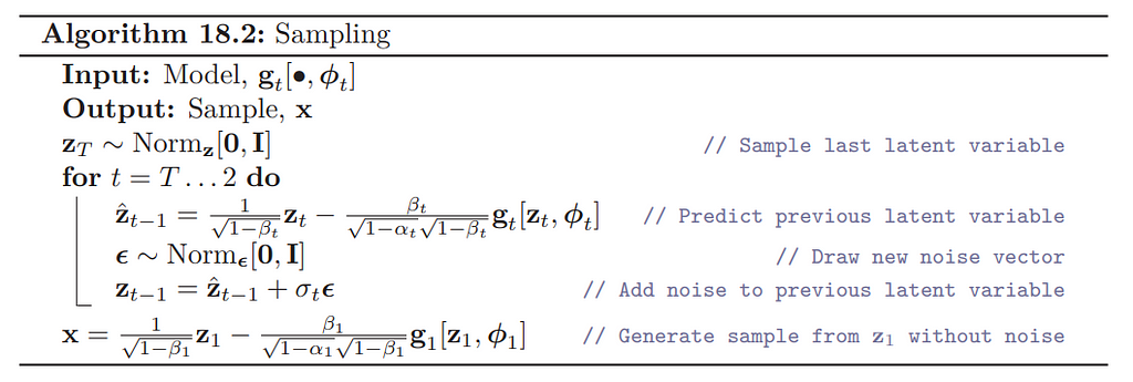
The sampling algorithm is summarized in the following:

1. Generate random noise from a standard normal distribution

For each timestep starting from our last timestep and moving backwards:

2. Update Z by estimating the reverse process distribution with mean parameterized by Z from the previous step and variance parameterized by the noise our model estimates at that timestep

3. Add a small amount of the noise back for stability (explanation below)

4. And repeat until we arrive at time step 0, our recovered image!

The algorithm to then sample and generate images might look mathematically complicated but it intuitively boils down to an iterative process where we start with pure noise, estimate the noise that theoretically was added at time step t, and subtract it. We do this until we arrive at our generated sample. The only small detail we should be mindful of is after we subtract the estimated noise, we add back a small amount of it to keep the process stable. For example, estimating and subtracting the total amount of noise in the beginning of the iterative process all at once leads to very incoherent samples, so in practice adding a bit of the noise back and iterating through every time step has empirically been shown to generate better samples.

The UNET

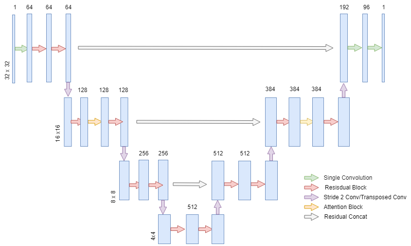
The authors of the DDPM paper used the UNET architecture originally designed for medical image segmentation to build a model to predict the noise for the diffusion reverse process. The model we are going to use in this tutorial is meant for 32×32 images perfect for datasets such as MNIST, but the model can be scaled to also handle data of much higher resolutions. There are many variations of the UNET, but the overview of the model architecture we will build is in the image below.

The UNET for DDPM is similar to the classic UNET because it contains both a down sampling stream and an up sampling stream that lightens the computational burden of the network, while also having skip connections between the two streams to merge the information from both the shallow and deep features of the model.

The main differences between the DDPM UNET and the classic UNET is that the DDPM UNET features attention in the 16×16 dimensional layers and sinusoidal transformer embeddings in every residual block. The meaning behind the sinusoidal embeddings is to tell the model which time step we are trying to predict the noise. This helps the model predict the noise at each time step by injecting positional information on where the model is on our noise schedule. For example, if we had a schedule of noise that had a lot of noise in certain time steps, the model understanding what time step it has to predict can help the model’s prediction on that noise for the corresponding time step. More general information on attention and embeddings can be found here [3] for those not already familiar with them from the transformer architecture.

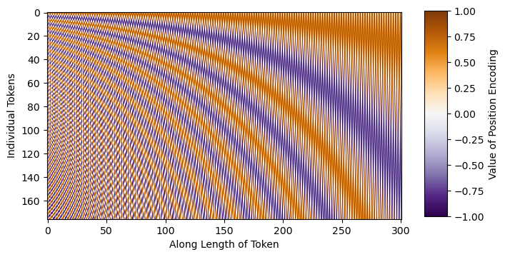
In our implementation of the model, we will start by defining our imports (possible pip install commands commented for reference) and coding our sinusoidal time step embeddings. Intuitively, the sinusoidal embeddings are different sin and cos frequencies that can be added directly to our inputs to give the model additional positional/sequential understanding. As you can see from the image below, each sinusoidal wave is unique which will give the model awareness on its location in our noise schedule.

# Imports
import torch
import torch.nn as nn
import torch.nn.functional as F
from einops import rearrange #pip install einops
from typing import List
import random
import math
from torchvision import datasets, transforms
from torch.utils.data import DataLoader 
from timm.utils import ModelEmaV3 #pip install timm 
from tqdm import tqdm #pip install tqdm
import matplotlib.pyplot as plt #pip install matplotlib
import torch.optim as optim
import numpy as np

class SinusoidalEmbeddings(nn.Module):
    def __init__(self, time_steps:int, embed_dim: int):
        super().__init__()
        position = torch.arange(time_steps).unsqueeze(1).float()
        div = torch.exp(torch.arange(0, embed_dim, 2).float() * -(math.log(10000.0) / embed_dim))
        embeddings = torch.zeros(time_steps, embed_dim, requires_grad=False)
        embeddings[:, 0::2] = torch.sin(position * div)
        embeddings[:, 1::2] = torch.cos(position * div)
        self.embeddings = embeddings

    def forward(self, x, t):
        embeds = self.embeddings[t].to(x.device)
        return embeds[:, :, None, None]

The residual blocks in each layer of the UNET will be equivalent to the ones used in the original DDPM paper. Each residual block will have a sequence of group-norm, the ReLU activation, a 3×3 “same” convolution, dropout, and a skip-connection.

# Residual Blocks
class ResBlock(nn.Module):
    def __init__(self, C: int, num_groups: int, dropout_prob: float):
        super().__init__()
        self.relu = nn.ReLU(inplace=True)
        self.gnorm1 = nn.GroupNorm(num_groups=num_groups, num_channels=C)
        self.gnorm2 = nn.GroupNorm(num_groups=num_groups, num_channels=C)
        self.conv1 = nn.Conv2d(C, C, kernel_size=3, padding=1)
        self.conv2 = nn.Conv2d(C, C, kernel_size=3, padding=1)
        self.dropout = nn.Dropout(p=dropout_prob, inplace=True)

    def forward(self, x, embeddings):
        x = x + embeddings[:, :x.shape[1], :, :]
        r = self.conv1(self.relu(self.gnorm1(x)))
        r = self.dropout(r)
        r = self.conv2(self.relu(self.gnorm2(r)))
        return r + x

In DDPM, the authors used 2 residual blocks per layer (resolution scale) of the UNET and for the 16×16 dimension layers, we include the classic transformer attention mechanism between the two residual blocks. We will now implement the attention mechanism for the UNET:

class Attention(nn.Module):
    def __init__(self, C: int, num_heads:int , dropout_prob: float):
        super().__init__()
        self.proj1 = nn.Linear(C, C*3)
        self.proj2 = nn.Linear(C, C)
        self.num_heads = num_heads
        self.dropout_prob = dropout_prob

    def forward(self, x):
        h, w = x.shape[2:]
        x = rearrange(x, 'b c h w -> b (h w) c')
        x = self.proj1(x)
        x = rearrange(x, 'b L (C H K) -> K b H L C', K=3, H=self.num_heads)
        q,k,v = x[0], x[1], x[2]
        x = F.scaled_dot_product_attention(q,k,v, is_causal=False, dropout_p=self.dropout_prob)
        x = rearrange(x, 'b H (h w) C -> b h w (C H)', h=h, w=w)
        x = self.proj2(x)
        return rearrange(x, 'b h w C -> b C h w')

The attention implementation is straight forward. We reshape our data such that the h*w dimensions are combined into a “sequence” dimension like the classic input for a transformer model and the channel dimension turns into the embedding feature dimension. In this implementation we utilize torch.nn.functional.scaled_dot_product_attention because this implementation contains flash attention, which is an optimized version of attention which is still mathematically equivalent to classic transformer attention. For more information on flash attention you can refer to these papers: [4], [5].

Finally at this point, we can define a complete layer of the UNET:

class UnetLayer(nn.Module):
    def __init__(self, 
            upscale: bool, 
            attention: bool, 
            num_groups: int, 
            dropout_prob: float,
            num_heads: int,
            C: int):
        super().__init__()
        self.ResBlock1 = ResBlock(C=C, num_groups=num_groups, dropout_prob=dropout_prob)
        self.ResBlock2 = ResBlock(C=C, num_groups=num_groups, dropout_prob=dropout_prob)
        if upscale:
            self.conv = nn.ConvTranspose2d(C, C//2, kernel_size=4, stride=2, padding=1)
        else:
            self.conv = nn.Conv2d(C, C*2, kernel_size=3, stride=2, padding=1)
        if attention:
            self.attention_layer = Attention(C, num_heads=num_heads, dropout_prob=dropout_prob)

    def forward(self, x, embeddings):
        x = self.ResBlock1(x, embeddings)
        if hasattr(self, 'attention_layer'):
            x = self.attention_layer(x)
        x = self.ResBlock2(x, embeddings)
        return self.conv(x), x

Each layer in DDPM as previously discussed has 2 residual blocks and may contain an attention mechanism, and we additionally pass our embeddings into each residual block. Also, we return both the downsampled or upsampled value as well as the value prior which we will store and use for our residual concatenated skip connections.

Finally, we can finish the UNET Class:

class UNET(nn.Module):
    def __init__(self,
            Channels: List = [64, 128, 256, 512, 512, 384],
            Attentions: List = [False, True, False, False, False, True],
            Upscales: List = [False, False, False, True, True, True],
            num_groups: int = 32,
            dropout_prob: float = 0.1,
            num_heads: int = 8,
            input_channels: int = 1,
            output_channels: int = 1,
            time_steps: int = 1000):
        super().__init__()
        self.num_layers = len(Channels)
        self.shallow_conv = nn.Conv2d(input_channels, Channels[0], kernel_size=3, padding=1)
        out_channels = (Channels[-1]//2)+Channels[0]
        self.late_conv = nn.Conv2d(out_channels, out_channels//2, kernel_size=3, padding=1)
        self.output_conv = nn.Conv2d(out_channels//2, output_channels, kernel_size=1)
        self.relu = nn.ReLU(inplace=True)
        self.embeddings = SinusoidalEmbeddings(time_steps=time_steps, embed_dim=max(Channels))
        for i in range(self.num_layers):
            layer = UnetLayer(
                upscale=Upscales[i],
                attention=Attentions[i],
                num_groups=num_groups,
                dropout_prob=dropout_prob,
                C=Channels[i],
                num_heads=num_heads
            )
            setattr(self, f'Layer{i+1}', layer)

    def forward(self, x, t):
        x = self.shallow_conv(x)
        residuals = []
        for i in range(self.num_layers//2):
            layer = getattr(self, f'Layer{i+1}')
            embeddings = self.embeddings(x, t)
            x, r = layer(x, embeddings)
            residuals.append(r)
        for i in range(self.num_layers//2, self.num_layers):
            layer = getattr(self, f'Layer{i+1}')
            x = torch.concat((layer(x, embeddings)[0], residuals[self.num_layers-i-1]), dim=1)
        return self.output_conv(self.relu(self.late_conv(x)))

The implementation is straight forward based on the classes we have already created. The only difference in this implementation is that our channels for the up-stream are slightly larger than the typical channels of the UNET. I found that this architecture trained more efficiently on a single GPU with 16GB of VRAM.

The Scheduler

Coding the noise/variance scheduler for DDPM is also very straightforward. In DDPM, our schedule will start, as previously mentioned, at 1e-4 and end at 0.02 and increase linearly.

class DDPM_Scheduler(nn.Module):
    def __init__(self, num_time_steps: int=1000):
        super().__init__()
        self.beta = torch.linspace(1e-4, 0.02, num_time_steps, requires_grad=False)
        alpha = 1 - self.beta
        self.alpha = torch.cumprod(alpha, dim=0).requires_grad_(False)

    def forward(self, t):
        return self.beta[t], self.alpha[t]

We return both the beta (variance) values and the alpha values since we the formulas for training and sampling use both based on their mathematical derivations.

def set_seed(seed: int = 42):
    torch.manual_seed(seed)
    torch.cuda.manual_seed_all(seed)
    torch.backends.cudnn.deterministic = True
    torch.backends.cudnn.benchmark = False
    np.random.seed(seed)
    random.seed(seed)

Additionally (not required) this function defines a training seed. This means that if you want to reproduce a specific training instance you can use a set seed such that the random weight and optimizer initializations are the same each time you use the same seed.

Training

For our implementation, we will create a model to generate MNIST data (hand written digits). Since these images are 28×28 by default in pytorch, we pad the images to 32×32 to follow the original paper trained on 32×32 images.

For optimization, we use Adam with initial learning rate of 2e-5. We also use EMA (Exponential Moving Average) to aid in generation quality. EMA is a weighted average of the model’s parameters that in inference time can create smoother, less noisy samples. For this implementation I use the library timm’s EMAV3 out of the box implementation with weight 0.9999 as used in the DDPM paper.

To summarize our training, we simply follow the psuedo-code above. We pick random time steps for our batch, noise our data in the batch based on our schedule at those time steps, and we input that batch of noised images into the UNET along with the time steps themselves to guide the sinusoidal embeddings. We use the formulas in the pseudo-code based on the “diffusion kernel” to noise the images. We then take our model’s prediction of how much noise we added and compare to the actual noise we added and optimize the mean squared error of the noise. We also implemented basic checkpointing to pause and resume training on different epochs.

def train(batch_size: int=64,
          num_time_steps: int=1000,
          num_epochs: int=15,
          seed: int=-1,
          ema_decay: float=0.9999,  
          lr=2e-5,
          checkpoint_path: str=None):
    set_seed(random.randint(0, 2**32-1)) if seed == -1 else set_seed(seed)

    train_dataset = datasets.MNIST(root='./data', train=True, download=False,transform=transforms.ToTensor())
    train_loader = DataLoader(train_dataset, batch_size=batch_size, shuffle=True, drop_last=True, num_workers=4)

    scheduler = DDPM_Scheduler(num_time_steps=num_time_steps)
    model = UNET().cuda()
    optimizer = optim.Adam(model.parameters(), lr=lr)
    ema = ModelEmaV3(model, decay=ema_decay)
    if checkpoint_path is not None:
        checkpoint = torch.load(checkpoint_path)
        model.load_state_dict(checkpoint['weights'])
        ema.load_state_dict(checkpoint['ema'])
        optimizer.load_state_dict(checkpoint['optimizer'])
    criterion = nn.MSELoss(reduction='mean')

    for i in range(num_epochs):
        total_loss = 0
        for bidx, (x,_) in enumerate(tqdm(train_loader, desc=f"Epoch {i+1}/{num_epochs}")):
            x = x.cuda()
            x = F.pad(x, (2,2,2,2))
            t = torch.randint(0,num_time_steps,(batch_size,))
            e = torch.randn_like(x, requires_grad=False)
            a = scheduler.alpha[t].view(batch_size,1,1,1).cuda()
            x = (torch.sqrt(a)*x) + (torch.sqrt(1-a)*e)
            output = model(x, t)
            optimizer.zero_grad()
            loss = criterion(output, e)
            total_loss += loss.item()
            loss.backward()
            optimizer.step()
            ema.update(model)
        print(f'Epoch {i+1} | Loss {total_loss / (60000/batch_size):.5f}')

    checkpoint = {
        'weights': model.state_dict(),
        'optimizer': optimizer.state_dict(),
        'ema': ema.state_dict()
    }
    torch.save(checkpoint, 'checkpoints/ddpm_checkpoint')

For inference, we exactly follow again the other part of the pseudo code. Intuitively, we are just reversing the forward process. We are starting from pure noise, and our now trained model can predict the estimated noise at each time step and can then generate brand new samples iteratively. Each different starting point for the noise, we can generate a different unique sample that is similar to our original data distribution but unique. The formulas for inference were not derived in this article but the reference linked in the beginning can help guide readers who want a deeper understanding.

Also note, I included a helper function to view the diffused images so you can visualize how well the model learned the reverse process.

def display_reverse(images: List):
    fig, axes = plt.subplots(1, 10, figsize=(10,1))
    for i, ax in enumerate(axes.flat):
        x = images[i].squeeze(0)
        x = rearrange(x, 'c h w -> h w c')
        x = x.numpy()
        ax.imshow(x)
        ax.axis('off')
    plt.show()

def inference(checkpoint_path: str=None,
              num_time_steps: int=1000,
              ema_decay: float=0.9999, ):
    checkpoint = torch.load(checkpoint_path)
    model = UNET().cuda()
    model.load_state_dict(checkpoint['weights'])
    ema = ModelEmaV3(model, decay=ema_decay)
    ema.load_state_dict(checkpoint['ema'])
    scheduler = DDPM_Scheduler(num_time_steps=num_time_steps)
    times = [0,15,50,100,200,300,400,550,700,999]
    images = []

    with torch.no_grad():
        model = ema.module.eval()
        for i in range(10):
            z = torch.randn(1, 1, 32, 32)
            for t in reversed(range(1, num_time_steps)):
                t = [t]
                temp = (scheduler.beta[t]/( (torch.sqrt(1-scheduler.alpha[t]))*(torch.sqrt(1-scheduler.beta[t])) ))
                z = (1/(torch.sqrt(1-scheduler.beta[t])))*z - (temp*model(z.cuda(),t).cpu())
                if t[0] in times:
                    images.append(z)
                e = torch.randn(1, 1, 32, 32)
                z = z + (e*torch.sqrt(scheduler.beta[t]))
            temp = scheduler.beta[0]/( (torch.sqrt(1-scheduler.alpha[0]))*(torch.sqrt(1-scheduler.beta[0])) )
            x = (1/(torch.sqrt(1-scheduler.beta[0])))*z - (temp*model(z.cuda(),[0]).cpu())

            images.append(x)
            x = rearrange(x.squeeze(0), 'c h w -> h w c').detach()
            x = x.numpy()
            plt.imshow(x)
            plt.show()
            display_reverse(images)
            images = []

def main():
    train(checkpoint_path='checkpoints/ddpm_checkpoint', lr=2e-5, num_epochs=75)
    inference('checkpoints/ddpm_checkpoint')

if __name__ == '__main__':
    main()

After training for 75 epochs with the experimental details listed above, we obtain these results:

At this point we have just coded DDPM from scratch in PyTorch!

Thanks for reading!

References

[1] DDPM https://arxiv.org/abs/2006.11239

[2] Understanding Deep Learning https://udlbook.github.io/udlbook/

[3] Attention is All You Need https://arxiv.org/abs/1706.03762

[4] Flash Attention https://arxiv.org/abs/2205.14135

[5] Flash Attention 2 https://arxiv.org/abs/2307.08691

Diffusion Model from Scratch in Pytorch was originally published in Towards Data Science on Medium, where people are continuing the conversation by highlighting and responding to this story.