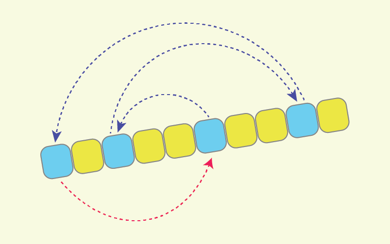
A sequence partitioning algorithm that does minimal rearrangements of values

1. Introduction
Sequence partitioning is a basic and frequently used algorithm in computer programming. Given a sequence of numbers “A”, and some value ‘p’ called pivot value, the purpose of a partitioning algorithm is to rearrange numbers inside “A” in such a way, so that all numbers less than ‘p’ come first, followed by the rest of the numbers.
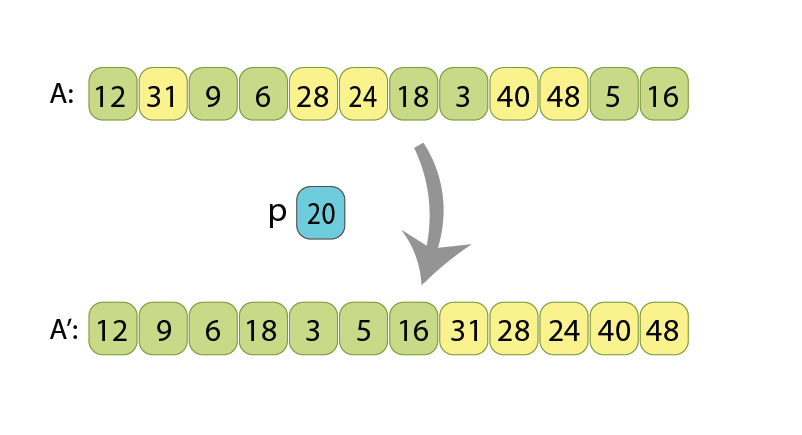
After the algorithm, all the values which are less than 20 (light green)
appear before the other values (yellow).
There are different applications of partitioning, but the most popular are:
- QuickSort — which is generally nothing more than a partitioning algorithm, called through recursion multiple times on different sub-arrays of given array, until it becomes sorted.
- Finding the median value of a given sequence — which makes use of partitioning in order to efficiently cut down the search range, and to ultimately find the median in expected linear time.
Sorting a sequence is an essential step to enable faster navigation over large amounts of data. Of the two common searching algorithms — linear search and binary search — the latter can only be used if the data in the array is sorted. Finding the median or k’th order statistic can be essential to understand the distribution of values in given unsorted data.
Currently there are different partitioning algorithms (also called — partition schemes), but the well-known ones are “Lomuto scheme” and “Hoare scheme”. Lomuto scheme is often intuitively easier to understand, while Hoare scheme does less rearrangements inside a given array, which is why it is often preferred in practice.
What I am going to suggest in this story is a new partition scheme called “cyclic partition”, which is similar to Hoare scheme, but does 1.5 times fewer rearrangements (value assignments) inside the array. Thus, as it will be shown later, the number of value assignments becomes almost equal to the number of the values which are initially “not at their place”, and should be somehow moved. That fact allows me to consider this new partition scheme as a nearly optimal one.
The next chapters are organized in the following way:
- In chapter 2 we will recall what is in-place partitioning (a property, which makes partitioning to be not a trivial task),
- In chapter 3 we will recall the widely used Hoare partitioning scheme,
- In chapter 4 I’ll present “cycles of assignments”, and we will see why some rearrangements of a sequence might require more value assignments, than other rearrangements of the same sequence,
- Chapter 5 will use some properties of “cycles of assignments”, and derive the new “cyclic partition” scheme, as an optimized variant of Hoare scheme,
- And finally, chapter 6 will present an experimental comparison between the Hoare scheme and cyclic partition, for arrays of small and large data types.
An implementation of Cyclic partition in the C++ language, as well as its benchmarking with the currently standard Hoare scheme, are present on GitHub, and are referenced at the end of this story [1].
2. Recalling in-place sequence partitioning
Partitioning a sequence will not be a difficult task, if the input and output sequences would reside in computer memory in 2 different arrays. If that would be the case, then one of methods might be to:
- Calculate how many values in “A” are less than ‘p’ (this will give us final length of the left part of output sequence),
- Scan the input array “A” from left to right, and append every current value “A[i]” either to the left part or to the right part, depending on whether it is less than ‘p’ or not.
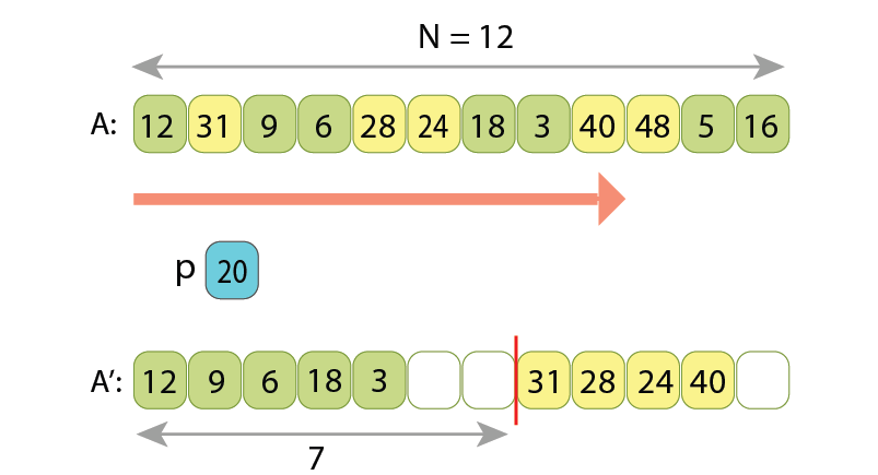
Here are presented a few states of running such algorithm:
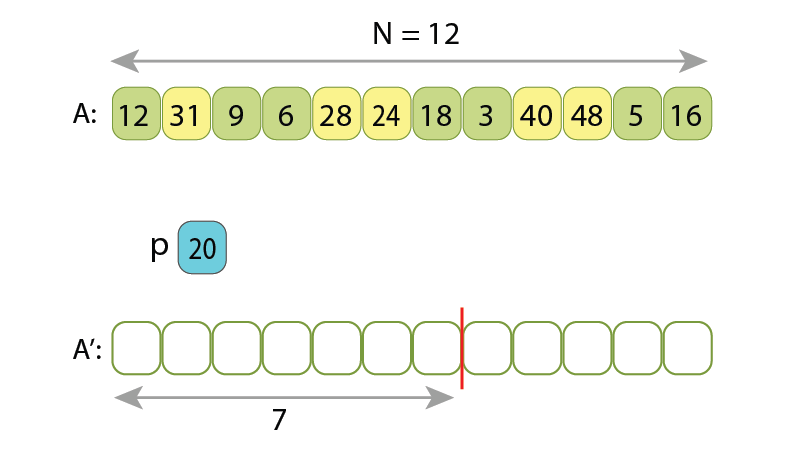
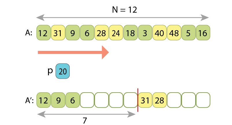
we append 3 of them to the left part of output sequence,
and the other 2 to its right part.
placing 5 of them in the left part of output sequence, and the other 4 to its right part.
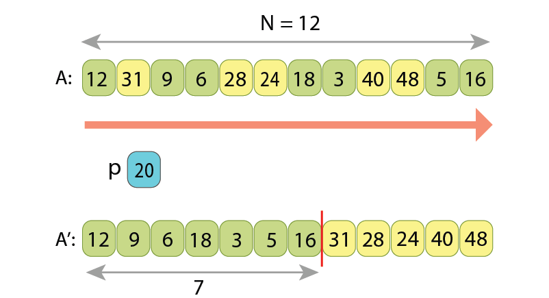
Note, the relative order of values in either left or right parts is preserved,
upon how they were originally written in the input array.
Other, shorter solutions also exist, such ones which have only one loop in the code.
Now, the difficulty comes when we want to not use any extra memory, so the input sequence will be transformed into the partitioned output sequence just by moving values inside the only array. By the way, such kind of algorithms which don’t use extra memory are called in-place algorithms.
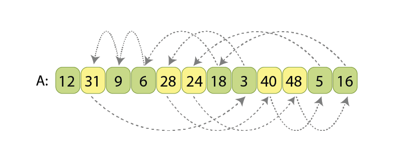
Presented order of values corresponds to the input state of the sequence, and arrows for every value show
if where to that value should be moved, in order for the entire sequence to become partitioned.
Before introducing my partitioning scheme, let’s review the existing and commonly used solution of in-place partitioning.
3. The currently used partitioning scheme
After observing a few implementations of sorting in standard libraries of various programming languages, it looks like the most widely used partitioning algorithm is the Hoare scheme. I found out that it is used for example in:
- “std::sort()” implementation in STL for C++,
- “Arrays.sort()” implementation in JDK for Java, for primitive data types.
In the partitioning based on the Hoare scheme, we scan the sequence simultaneously from both ends towards each other, searching in the left part such a value A[i] which is greater or equal to ‘p’, and searching in the right part such a value A[j] which is less than ‘p’. Once found, we know that those two values A[i] and A[j] are kind of “not at their proper places” (remember, the partitioned sequence should have the values less than ‘p’ coming first, and only then all the other values which are greater or equal to ‘p’), so we just swap A[i] and A[j]. After the swap, we continue the same way, simultaneously scanning array “A” with indexes i and j, until they become equal. Once they are, partitioning is completed.
Let’s observe the Hoare scheme on another example:
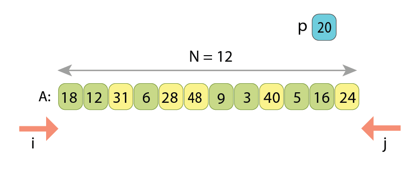
Index i starts scanning from 0 upwards, and index j starts scanning from “N-1” downwards.
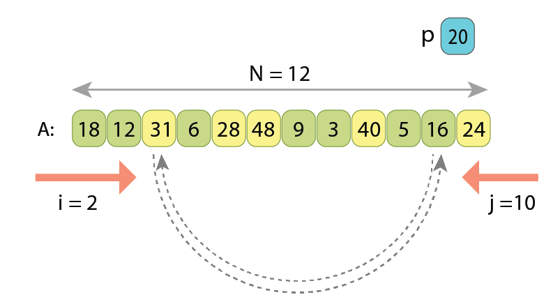
we meet another value “A[10]=16” which is less than ‘p’. Those 2 are going to be swapped.
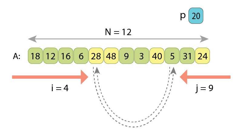
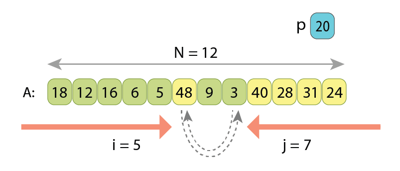
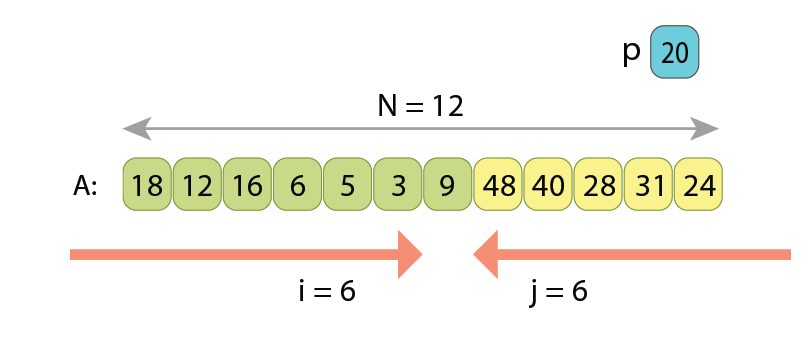
If writing the pseudo-code of partitioning by the Hoare scheme, we will have the following:
// Partitions sequence A[0..N) with pivot value 'p'
// upon Hoare scheme, and returns index of the first value
// of the resulting right part.
function partition_hoare( A[0..N) : Array of Integers, p: Integer ) : Integer
    i := 0
    j := N-1
    while true
        // Move left index 'i', as much as needed
        while i < j and A[i] < p
            i := i+1
        // Move right index 'j', as much as needed
        while i < j and A[j] >= p
            j := j-1
        // Check for completion
        if i >= j
            if i == j and A[i] < p
                return i+1  // "A[i]" also refers to left part
            else
                return i  // "A[i]" refers to right part
        // Swap "A[i]" and "A[j]"
        tmp := A[i]
        A[i] := A[j]
        A[j] := tmp
        // Advance by one both 'i' and 'j'
        i := i+1
        j := j-1
Here in lines 5 and 6 we set up start indexes for the 2 scans.
Lines 8–10 search from left for such a value, which should belong to the right part, after partitioning.
Similarly, lines 11–13 search from right for such a value, which should belong to the left part.
Lines 15–19 check for completion of the scans. Once indexes ‘i’ and ‘j’ meet, there are 2 cases: either “A[i]” belongs to the left part or to the right part. Depending on that, we return either ‘i’ or ‘i+1’, as return value of the function should be the start index of the right part.
Next, if the scans are not completed yet, lines 20–23 do swap those 2 values which are not at their proper places.
And finally, lines 24–26 advance the both indexes, in order to not re-check the already swapped values.
The time complexity of the algorithm is O(N), regardless of where the 2 scans will meet each other, as together they always scan N values.
An important note here, if the array “A” has ‘L’ values which are “not at their places”, and should be swapped, then acting by Hoare scheme we will do “3*L/2” assignments, because swapping 2 values requires 3 assignments:
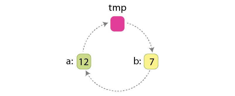
Those assignments are:
tmp := a
a := b
b := tmp
Let me also emphasize here that ‘L’ is always an even number. That is because for every value “A[i]>=p” originally residing at the left area, there is another value “A[j]<p” originally residing at the right area, the ones which are being swapped. So, every swap rearranges 2 such values, and all rearrangements in Hoare scheme are being done only through swaps. That’s why the ‘L’ — the total number of values to be rearranged, is always an even number.
4. Cycles of assignments
This chapter might look as a deviation from the agenda of the story, but actually it isn’t, as we will need the knowledge about cycles of assignments in the next chapter, when optimizing the Hoare partitioning scheme.
Assume that we want to somehow rearrange the order of values in given sequence “A”. This should not necessarily be a partitioning, but any kind of rearrangement. Let me show that some rearrangements require more assignments than some others.
Case #1: Cyclic left-shift of a sequence
How many assignments should be done if we want to cyclic left shift the sequence “A” by 1 position?
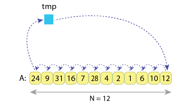
We see that the number of assignments needed is N+1=13, as we need to:
1) store “A[0]” in the temporary variable “tmp”, then
2) “N-1” times assign the right adjacent value to the current one, and finally
3) assign “tmp” to the last value of the sequence “A[N-1]”.
The needed operations to do that are:
tmp := A[0]
A[0] := A[1]
A[1] := A[2]
...
A[9] := A[10]
A[10] := A[11]
A[11] := tmp
… which results in 13 assignments.
Case #2: Cyclic left-shift by 3 positions
In the next example we still want to do a cyclic left shift of the same sequence, but now by 3 positions to the left:
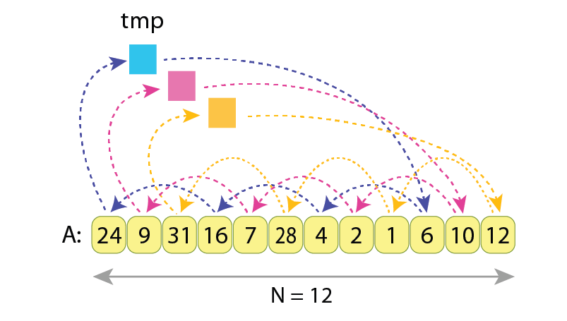
We see that the values A[0], A[3], A[6] and A[9] are being exchanged between each other (blue arrows),
as well as values A[1], A[4], A[7] and A[10] do (pink arrows),
and as the values A[2], A[5], A[8] and A[11] do exchange only between each other (yellow arrows).
The “tmp” variable is being assigned to and read from 3 times.
Here we have 3 independent chains / cycles of assignments, each of length 4.
In order to properly exchange values between A[0], A[3], A[6] and A[9], the needed actions are:
tmp := A[0]
A[0] := A[3]
A[3] := A[6]
A[6] := A[9]
A[9] := tmp
… which makes 5 assignments. Similarly, exchanging values inside groups (A[1], A[4], A[7], A[10]) and (A[2], A[5], A[8], A[11]) will require 5 assignments each. And adding all that together gives 5*3=15 assignments required to cyclic left shift by 3 the sequence “A”, having N=12 values.
Case #3: Reversing a sequence
When reversing the sequence “A” of length ’N’, the actions performed are:
- swap its first value with the last one, then
- swap the second value with the second one from right,
- swap the third value with the third one from right,
- … and so on.
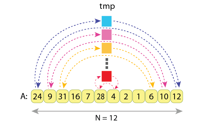
We see that the values in pairs (A[0], A[11]), (A[1], A[10]), (A[2], A[9]), etc, are being swapped, independently from each other. The variable “tmp” is being assigned to and read from 6 times.
As every swap requires 3 assignments, and as for reversing entire sequence “A” we need to do ⌊N/2⌋ swaps, the total number of assignments results in:
3*⌊N/2⌋ = 3*⌊12/2⌋ = 3*6 = 18
And the exact sequence of assignments needed to do the reverse of “A” is:
tmp := A[0]    // Cycle 1
A[0] := A[11]
A[11] := tmp
tmp := A[1]    // Cycle 2
A[1] := A[10]
A[10] := tmp

...

tmp := A[5]    // Cycle 6
A[5] := A[6]
A[6] := tmp
Summary
We have seen that rearranging values of the same sequence “A” might require different number of assignments, depending on how exactly the values are being rearranged.
In the presented 3 examples, the sequence always had length of N=12, but the number of required assignments was different:

More precisely, the number of assignments is equal to N+C, where “C” is the number of cycles, which originate during the rearrangement. Here by saying “cycle” I mean such a subset of variables of “A”, values of which are being rotated among each other.
In our case 1 (left shift by 1) we had only C=1 cycle of assignments, and all variables of “A” did participate in that cycle. That’s why overall number of assignments was:
N+C = 12+1 = 13.
In the case 2 (left shift by 3) we had C=3 cycles of assignments, with:
— first cycle within variables (A[0], A[3], A[6], A[9]),
— second cycle applied to variables (A[1], A[4], A[7], A[10]) and
— third cycle applied to variables (A[2], A[5], A[8], A[11]).
That’s why the overall number of assignments was:
N+C = 12+3 = 15.
And in our case 3 (reversing) we had ⌊N/2⌋ = 12/2 = 6 cycles. Those all were the shortest possible cycles, and were applied to pairs (A[0], A[11]), (A[1], A[10]), … and so on. That’s why the overall number of assignments was:
N+C = 12+6 = 18.
Surely, in the presented examples the absolute difference in number of assignments is very small, and it will not play any role when writing high-performance code. But that is because we were considering a very short array of length “N=12”. For longer arrays, those differences in numbers of assignments will grow proportionally to N.
Concluding this chapter, let’s keep in mind that the number of assignments needed to rearrange a sequence grows together with number of cycles, introduced by such rearrangement. And if we want to have a faster rearrangement, we should try to do it by such a scheme, which has the smallest possible number of cycles of assignments.
5. Optimizing the Hoare partitioning scheme
Now let’s observe the Hoare partitioning scheme once again, this time paying attention to how many cycles of assignments it introduces.
Let’s assume we have the same array “A” of length N, and a pivot value ‘p’ according to which the partitioning must be made. Also let’s assume that there are ‘L’ values in the array which should be somehow rearranged, in order to bring “A” into a partitioned state. It turns out that Hoare partitioning scheme rearranges those ‘L’ values in the slowest possible way, because it introduces the maximal possible number of cycles of assignments, with every cycle consisting of only 2 values.
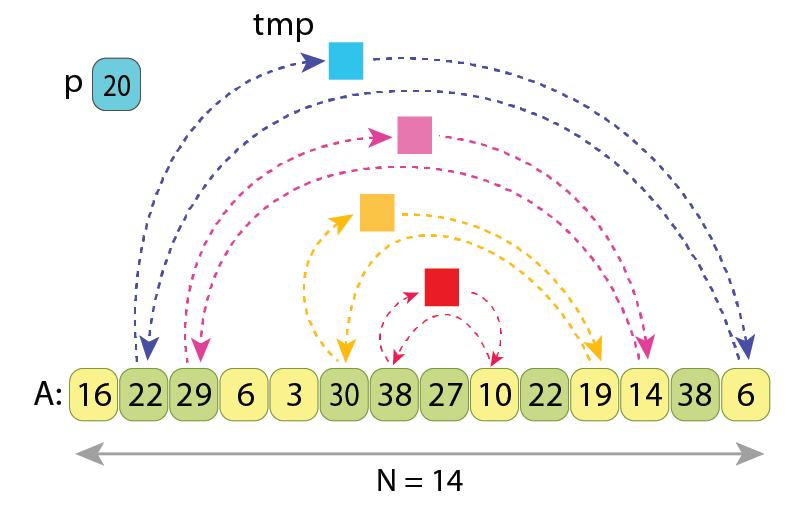
arrows are coming (or going from).
Hoare partitioning scheme introduces “L/2=4” cycles of assignments, each acting on just 2 values.
Moving 2 values over a cycle of length 2, which is essentially swapping them, requires 3 assignments. So the overall number of values assignments is “3*L/2” for the Hoare partitioning scheme.
The idea which lies beneath the optimization that I am going to describe, comes from the fact that after partitioning a sequence, we are generally not interested in relative order of the values “A[i]<p”, which should finish at the left part of partitioned sequence, as well as we are not interested in the relative order of the ones, which should finish at the right part. The only thing that we are interested in, is for all values less than ‘p’ to come before the other ones. This fact allows us to alter the cycles of assignments in Hoare scheme, and to come up with only 1 cycle of assignments, containing all the ‘L’ values, which should somehow be rearranged.
Let me first describe the altered partitioning scheme with the help of the following illustration:
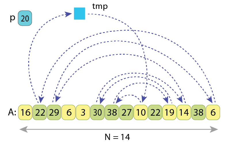
As the pivot “p=20” is not changed, the “L=8” values which should be rearranged are also the same.
All the arrows represent the only cycle of assignments in the new scheme.
After moving all the ‘L’ values upon it, we will end up with an alternative partitioned sequence.
So what are we doing here?
- As in the original Hoare scheme, at first we scan from the left and find such value “A[i]>=p” which should go to the right part. But instead of swapping it with some other value, we just remember it: “tmp := A[i]”.
- Next we scan from right and find such value “A[j]<p” which should go to the left part. And we just do the assignment “A[i] := A[j]”, without loosing the value of “A[i]”, as it is already stored in “tmp”.
- Next we continue the scan from left, and find such value “A[i]>=p” which also should go to the right part. So we do the assignment “A[j] := A[i]”, without loosing value “A[j]”, as it is already assigned to the previous position of ‘i’.
- This pattern continues, and once indexes i and j meet each other, it remains to place some value greater than ‘p’ to “A[j]”, we just do “A[j] := tmp”, as initially the variable “tmp” was holding the first value from left, greater than ‘p’. The partitioning is completed.
As we see, here we have only 1 cycle of assignments which goes over all the ‘L’ values, and in order to properly rearrange them it requires just “L+1” value assignments, compared to the “3*L/2” assignments of Hoare scheme.
I prefer to call this new partitioning scheme a “Cyclic partition”, because all the ‘L’ values which should be somehow rearranged, now reside on a single cycle of assignments.
Here is the pseudo-code of the Cyclic partition algorithm. Compared to the pseudo-code of Hoare scheme the changes are insignificant, but now we always do 1.5x fewer assignments.
// Partitions sequence A[0..N) with pivot value 'p'
// by "cyclic partition" scheme, and returns index of
// the first value of the resulting right part.
function partition_cyclic( A[0..N) : Array of Integers, p: Integer ) : Integer
    i := 0
    j := N-1
    // Find the first value from left, which is not on its place
    while i < N and A[i] < p
        i := i+1
    if i == N
        return N  // All N values go to the left part
    // The cycle of assignments starts here
    tmp := A[i]  // The only write to 'tmp' variable
    while true
        // Move right index 'j', as much as needed
        while i < j and A[j] >= p
            j := j-1
        if i == j  // Check for completion of scans
            break
        // The next assignment in the cycle
        A[i] := A[j]
        i := i+1
        // Move left index 'i', as much as needed
        while i < j and A[i] < p
            i := i+1
        if i == j  // Check for completion of scans
            break
        // The next assignment in the cycle
        A[j] := A[i]
        j := j-1
    // The scans have completed
    A[j] := tmp  // The only read from 'tmp' variable
    return j
Here lines 5 and 6 set up the start indexes for both scans (‘i’ — from left to right, and ‘j’ — from right to left).
Lines 7–9 search from left for such a value “A[i]”, which should go to the right part. If it turns out that there is no such value, and all N items belong to the left part, lines 10 and 11 report that and finish the algorithm.
Otherwise, if such value was found, at line 13 we remember it in the ‘tmp’ variable, thus opening a slot at index ‘i’ for placing another value there.
Lines 15–19 search from right for such a value “A[j]” which should be moved to the left part. Once found, lines 20–22 place it into the empty slot at index ‘i’, after which the slot at index ‘j’ becomes empty, and waits for another value.
Similarly, lines 23–27 search from left for such a value “A[i]” which should be moved to the right part. Once found, lines 28–30 place it into the empty slot at index ‘j’, after which the slot at index ‘i’ again becomes empty, and waits for another value.
This pattern is continued in the main loop of the algorithm, at lines 14–30.
Once indexes ‘i’ and ‘j’ meet each other, we have an empty slot there, and lines 31 and 32 assign the originally remembered value in ‘tmp’ variable there, so the index ‘j’ becomes the first one to hold such value which belongs to the right part.
The last line returns that index.
This way we can write 2 assignments of the cycle together in the loop’s body, because as it was proven in chapter 3, ‘L’ is always an even number.
Time complexity of this algorithm is also O(N), as we still scan the sequence from both ends. It just does 1.5x less value assignments, so the speed-up is reflected only in the constant factor.
An implementation of Cyclic partition in the C++ language is present on GitHub, and is referenced at the end of this story [1].
I also want to show that the value ‘L’ figuring in the Hoare scheme can’t be lowered, regardless of what partitioning scheme we use. Assume that after partitioning, the length of the left part will be “left_n”, and length of the right part will be “right_n”. Now, if looking at the left-aligned “left_n”-long area of the original unpartitioned array, we will find some ‘t1’ values there, which are not at their final places. So those are such values which are greater or equal to ‘p’, and should be moved to the right part anyway.
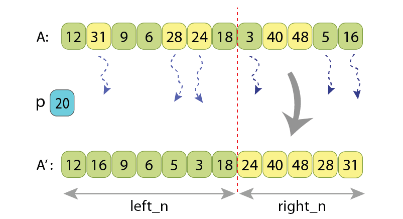
Length of the left part is “left_n=7” and length of the right part is “right_n=5”.
Among the first 7 values of the unpartitioned sequence there are “t1=3” of them
which are greater than “p=20” (the yellow ones), and should be somehow moved to the right part.
And among the last 5 values of the unpartitioned sequence there are “t2=3” of them
which are less than ‘p’ (the light green ones), and should be somehow moved to the left part.
Similarly, if looking at the right-aligned “right_n”-long area of the original unpartitioned array, we will find some ‘t2’ values there, which are also not at their final places. Those are such values which are less than ‘p’, and should be moved to the left part. We can’t move less than ‘t1’ values from left to right, as well as we can’t move less than ‘t2’ values from right to left.
In the Hoare partitioning scheme, the ‘t1’ and ‘t2’ values are the ones which are swapped between each other. So there we have:
t1 = t2 = L/2,
or
t1 + t2 = L.
Which means that ‘L’ is actually the minimal amount of values which should be somehow rearranged, in order for the sequence to become partitioned. And the Cyclic partition algorithm rearranges them doing just “L+1” assignments. That’s why I allow myself to call this new partitioning scheme as “nearly optimal”.
6. Experimental results
It is already proven that the new partitioning scheme is doing fewer assignments of values, so we can expect it to run faster. However, before publishing the algorithm I wanted to collect the results also in an experimental way.
I have compared the running times when partitioning by the Hoare scheme and by Cyclic partition. All the experiments were performed on randomly shuffled arrays.
The parameters by which the experiments were different are:
- N — length of the array,
- “left_part_percent” — percent of length of the left part (upon N), which results after partitioning,
- running on array of primitive data type variables (32-bit integers) vs. on array of some kind of large objects (256-long static arrays of 16-bit integers).
I want to clarify why I found it necessary to run partitioning both on arrays of primitive data types, and on arrays of large objects. Here, by saying “large object” I mean such values, which occupy much more memory, compared to primitive data types. When partitioning primitive data types, assigning one variable to another will work as fast as almost all other instructions used in both algorithms (like incrementing an index or checking condition of the loop). Meanwhile when partitioning large objects, assigning one such object to another will take significantly more time, compared to other used instructions, and that is when we are interested to reduce the overall number of value assignments as much as that is possible.
I’ll explain why I decided to run different experiments with different values of “left_part_percent” a bit later in this chapter.
The experiments were performed with Google Benchmark, under the following system:
CPU: Intel Core i7–11800H @ 2.30GHz
RAM: 16.0 GB
OS: Windows 11 Home, 64-bit
Compiler: MSVC 2022 ( /O2 /Ob2 /MD /GR /Gd )
Partitioning arrays of a primitive data type
Here are the results of running partition algorithms on arrays of primitive data type — 32 bit integer:

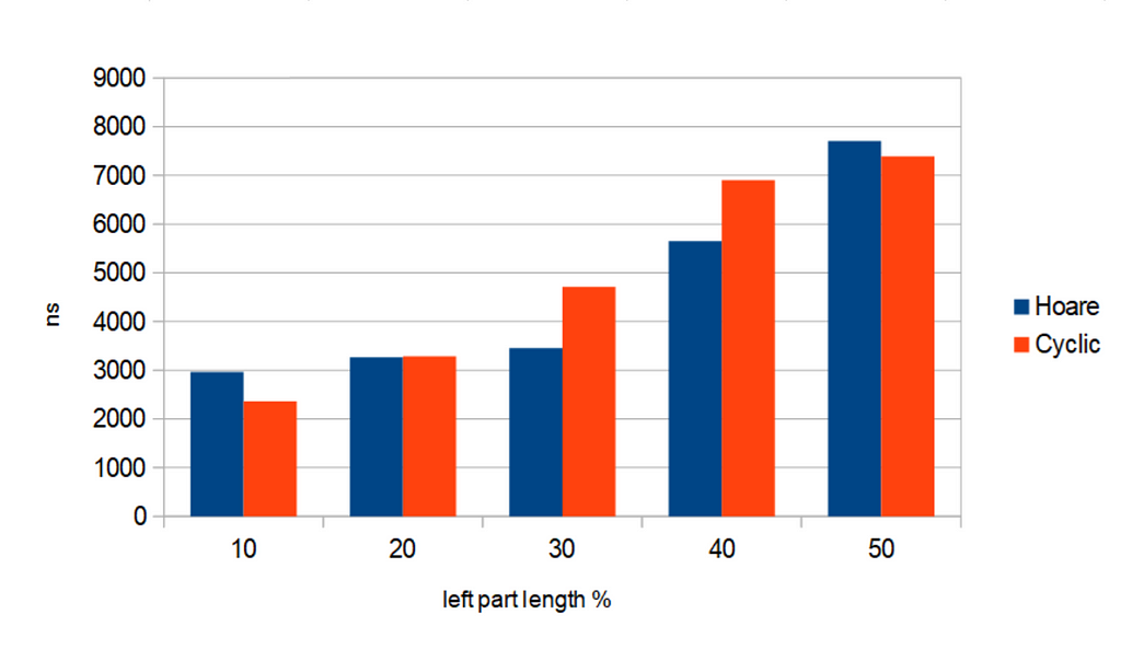
Blue bars correspond to partitioning by Hoare scheme,
while red bars correspond to the Cyclic partition algorithm.
Partitioning algorithms are run for 5 different cases, based on “left_part_percent” — percent of the left part of array (upon N), that will appear after partitioning. The time is presented in nanoseconds.
We see that there is no obvious correlation between value of “left_part_percent” and relative difference in running times of the 2 algorithms. This kind of behavior is expected.
Partitioning arrays of “large objects”
And here are the results of running the 2 partitioning algorithms on array of so called “large objects” — each of which is an 256-long static array of 16-bit random integers.

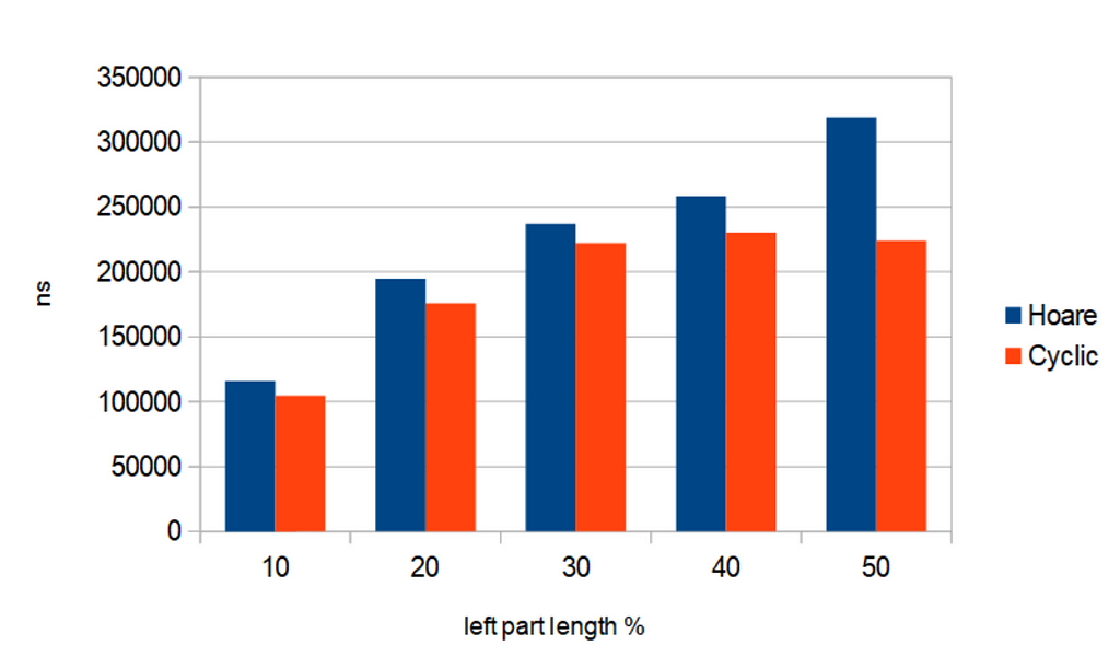
(256-long static arrays of random 16-bit integers), having length N=10’000.
Blue bars correspond to partitioning by Hoare scheme,
while red bars correspond to the Cyclic partition algorithm.
Partitioning algorithms are run for 5 different cases, based on “left_part_percent” — percent of the left part of array (upon N), that will appear after partitioning. The time is presented in nanoseconds.
Now we see an obvious correlation: Cyclic partition outperforms the Hoare scheme as more, as the “left_part_percent” is closer to 50%. In other words, Cyclic partition works relatively faster when after partitioning the left and right parts of the array appear to have closer lengths. This is also an expected behavior.
Explanation of the results
— Why does partitioning generally take longer, when “left_part_percent” is closer to 50%?
Let’s imagine for a moment a corner case — when after partitioning almost all values appear in left (or right) part. This will mean that almost all values of the array were less (or greater) than the pivot value. And it will mean that during the scan, all those values were considered to be already at their final positions, and very few assignments of values were performed. If trying to imagine the other case — when after partitioning the left and right parts appear to have almost equal length, it will mean that a lot of value assignments were performed (as initially all the values were randomly shuffled in the array).
— When looking at partitioning of “large objects”, why does the difference in running time of the 2 algorithms become greater when “left_part_percent” gets closer to 50%?
The previous explanation shows that when “left_part_percent” gets closer to 50%, there arises need to do more assignments of values in the array. In previous chapters we also have shown that Cyclic partition always makes 1.5x less value assignments, compared to Hoare scheme. So that difference of 1.5 times brings more impact on overall running time when we generally need to do more rearrangements of values in the array.
— Why is the absolute time (in nanoseconds) greater when partitioning “large objects”, rather than when partitioning 32-bit integers?
This one is simple — because assigning one “large object” to another takes much more time, than assigning one primitive data type to another.
I also run all the experiments on arrays with different lengths, but the overall picture didn’t change.
7. Conclusion
In this story I introduced an altered partitioning scheme, called “Cyclic partition”. It always makes 1.5 times fewer value assignments, compared to the currently used Hoare partitioning scheme.
Surely, when partitioning a sequence, value assignment is not the only type of operation performed. Besides it, partitioning algorithms check values of input sequence “A” for being less or greater than the pivot value ‘p’, as well as they do increments and decrements of indexes over “A”. The amounts of comparisons, increments and decrements are not affected by introducing “cyclic partition”, so we can’t just expect it to run 1.5x faster. However, when partitioning an array of complex data types, where value assignment is significantly more time-consuming than simply incrementing or decrementing an index, the overall algorithm can actually run up to 1.5 times faster.
The partitioning procedure is the main routine of the QuickSort algorithm, as well as of the algorithm for finding the median of an unsorted array, or finding its k-th order statistic. So we can also expect for those algorithms to have a performance gain up to 1.5 times, when working on complex data types.
My gratitudes to:
— Roza Galstyan, for reviewing the draft of the story and suggesting useful enhancements,
— David Ayrapetyan, for the spell check ( https://www.linkedin.com/in/davidayrapetyan/ ),
— Asya Papyan, for careful design of all used illustrations ( https://www.behance.net/asyapapyan ).
If you enjoyed this story, feel free to find and connect me on LinkedIn ( https://www.linkedin.com/in/tigran-hayrapetyan-cs/ ).
All used images, unless otherwise noted, are designed by request of the author.
References:
[1] — Implementation of Cyclic partition in C++ : https://github.com/tigranh/cyclic_partition
Cyclic Partition: An Up to 1.5x Faster Partitioning Algorithm was originally published in Towards Data Science on Medium, where people are continuing the conversation by highlighting and responding to this story.
Originally appeared here:
Cyclic Partition: An Up to 1.5x Faster Partitioning Algorithm
Go Here to Read this Fast! Cyclic Partition: An Up to 1.5x Faster Partitioning Algorithm
