Chi-Squared Test: Revealing Hidden Patterns in Your Data

Unlock hidden patterns in your data with the chi-squared test in Python.

Part 1: What is Chi-Squared Test?

When discussing hypothesis testing, there are many approaches we can take, depending on the particular cases. Common tests like the z-test and t-test are the go-to methods to test our hypotheses (null and alternative hypotheses). The metric we want to test differs depending on the problem. Usually, in generating hypotheses, we involve population mean or population proportion as the metric to state them. Let’s say we want to test whether the population proportion of the students who took the math test who got 75 is more than 80%. Let the null hypothesis be denoted by H0, and the alternative hypothesis be denoted by H1; we generate the hypotheses by:

After that, we should see our data, whether the population variance is known or unknown, to decide which test statistic formula we should use. In this case, we use z-statistic for proportion formula. To calculate the test statistics from our sample, first, we estimate the population proportion by dividing the total number of students who got 75 by the total number of students who participated in the test. After that, we plug in the estimated proportion to calculate the test statistic using the test statistic formula. Then, we determine from the test statistic result if it will reject or fail to reject the null hypothesis by comparing it with the rejection region or p-value.

But what if we want to test different cases? What if we make inferences about the proportion of the group of students (e.g., class A, B, C, etc.) variable in our dataset? What if we want to test if there is any association between groups of students and their preparation before the exam (are they doing extra courses outside school or not)? Is it independent or not? What if we want to test categorical data and infer their population in our dataset? To test that, we’ll be using the chi-squared test.

The chi-squared test is crafted to help us draw conclusions about categorical data that fall into different categories. It compares each category’s observed frequencies (counts) to the expected frequencies under the null hypothesis. Denoted as X², chi-squared has a distribution, namely chi-squared distribution, allowing us to determine the significance of the observed deviations from expected values.

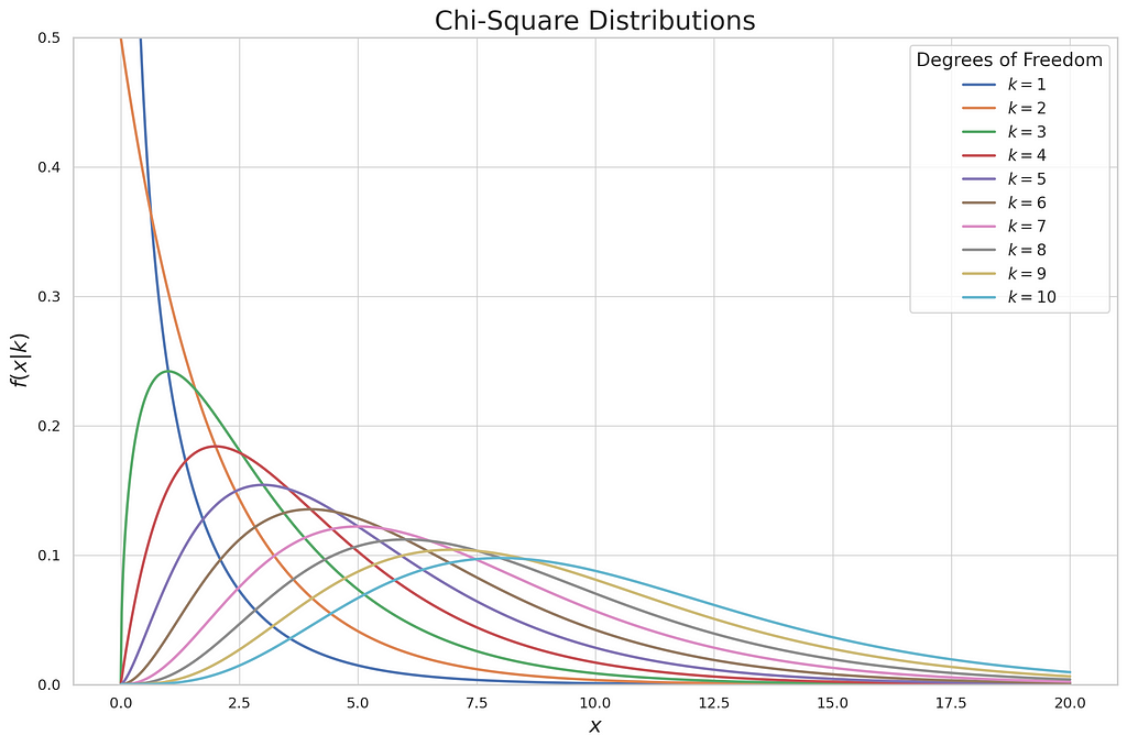
The plot describes the continuous distribution of each degree of freedom in the chi-squared test. In the chi-squared test, to prove whether we will reject or fail to reject the null hypothesis, we don’t use the z or t table to decide, but we use the chi-squared table. It lists probabilities of selected significance level and degree of freedom of chi-squared. There are two types of chi-squared tests, the chi-squared goodness-of-fit test and the chi-squared test of a contingency table. Each of these types has a different purpose when tackling the hypothesis test. In parallel with the theoretical approach of each test, I’ll show you how to demonstrate those two tests in practical examples.

Part 2: Chi-squared goodness-of-fit test

This is the first type of the chi-squared test. This test analyzes a group of categorical data from a single categorical variable with k categories. It is used to specifically explain the proportion of observations in each category within the population. For example, we surveyed 1000 students who got at least 75 on their math test. We observed that from 5 groups of students (Class A to E), the distribution is like this:

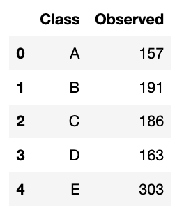
We will do it in both manual and Python ways. Let’s start with the manual one.

Form Hypotheses

As we know, we have already surveyed 1000 students. I want to test whether the population proportions in each class are equal. The hypotheses will be:

Test Statistic

The test statistic formula for the chi-squared goodness-of-fit test is like this:

Where:

• k: number of categories
• fi: observed counts
• ei: expected counts

We already have the number of categories (5 from Class A to E) and the observed counts, but we don’t have the expected counts yet. To calculate that, we should reflect on our hypotheses. In this case, I assume that all class proportions are the same, which is 20%. We will make another column in the dataset named Expected. We calculate it by multiplying the total number of observations by the proportion we choose:

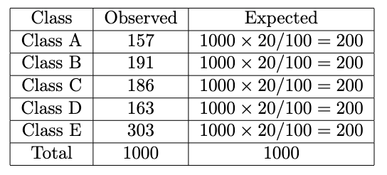
Now we plug in the formula like this for each observed and expected value:

We already have the test statistic result. But how do we decide whether it will reject or fail to reject the null hypothesis?

Decision Rule

As mentioned above, we’ll use the chi-squared table to compare the test statistic. Remember that a small test statistic supports the null hypothesis, whereas a significant test statistic supports the alternative hypothesis. So, we should reject the null hypothesis when the test statistic is substantial (meaning this is an upper-tailed test). Because we do this manually, we use the rejection region to decide whether it will reject or fail to reject the null hypothesis. The rejection region is defined as below:

Where:

• α: Significance Level
• k: number of categories

The rule of thumb is: If our test statistic is more significant than the chi-squared table value we look up, we reject the null hypothesis. We’ll use the significance level of 5% and look at the chi-squared table. The value of chi-squared with a 5% significance level and degrees of freedom of 4 (five categories minus 1), we get 9.49. Because our test statistic is way more significant than the chi-squared table value (70.52 > 9.49), we reject the null hypothesis at a 5% significance level. Now, you already know how to perform the chi-squared goodness-of-fit test!

Python Approach

This is the Python approach to the chi-squared goodness-of-fit test using SciPy:

import pandas as pd
from scipy.stats import chisquare

# Define the student data
data = {
    'Class': ['A', 'B', 'C', 'D', 'E'],
    'Observed': [157, 191, 186, 163, 303]
}

# Transform dictionary into dataframe
df = pd.DataFrame(data)

# Define the null and alternative hypotheses
null_hypothesis = "p1 = 20%, p2 = 20%, p3 = 20%, p4 = 20%, p5 = 20%"
alternative_hypothesis = "The population proportions do not match the given proportions"

# Calculate the total number of observations and the expected count for each category
total_count = df['Observed'].sum()
expected_count = total_count / len(df)  # As there are 5 categories

# Create a list of observed and expected counts
observed_list = df['Observed'].tolist()
expected_list = [expected_count] * len(df)

# Perform the Chi-Squared goodness-of-fit test
chi2_stat, p_val = chisquare(f_obs=observed_list, f_exp=expected_list)

# Print the results
print(f"nChi2 Statistic: {chi2_stat:.2f}")
print(f"P-value: {p_val:.4f}")

# Print the conclusion
if p_val < 0.05:
    print("Reject the null hypothesis: The population proportions do not match the given proportions.")
else:
    print("Fail to reject the null hypothesis: The population proportions match the given proportions.")

Using the p-value, we also got the same result. We reject the null hypothesis at a 5% significance level.

Part 3: Chi-squared test of a contingency table

We already know how to make inferences about the proportion of one categorical variable. But what if I want to test whether two categorical variables are independent?

To test that, we use the chi-squared test of the contingency table. We will utilize the contingency table to calculate the test statistic value. A contingency table is a cross-tabulation table that classifies counts summarizing the combined distribution of two categorical variables, each having a finite number of categories. From this table, you can determine if the distribution of one categorical variable is consistent across all categories of the other categorical variable.

I will explain how to do it manually and using Python. In this example, we sampled 1000 students who got at least 75 on their math test. I want to test whether the variable of a group of students and the variable of the students who have taken the supplementary course (Taken or Not) outside the school before the test is independent. The distribution is like this:

Form Hypotheses

To generate these hypotheses is very simple. We define the hypotheses as:

Test Statistic

This is the hardest part. In handling real data, I suggest you use Python or other statistical software directly because the calculation is too complicated if we do it manually. But because we want to know the approach from the formula, let’s do the manual calculation. The test statistic of this test is:

Where:

• r = number of rows
• c = number of columns
• fij: the observed counts
• eij = (i th row total * j th row total)/sample size

Recall Figure 9, those values are just observed ones. Before we use the test statistic formula, we should calculate the expected counts. We do that by:

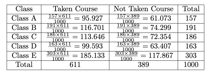
Now we get the observed and expected counts. After that, we will calculate the test statistic by:

Decision Rule

We already have the test statistic; now we compare it with the rejection region. The rejection region for the contingency table test is defined by:

Where:

• α: Significance Level
• r = number of rows
• c = number of columns

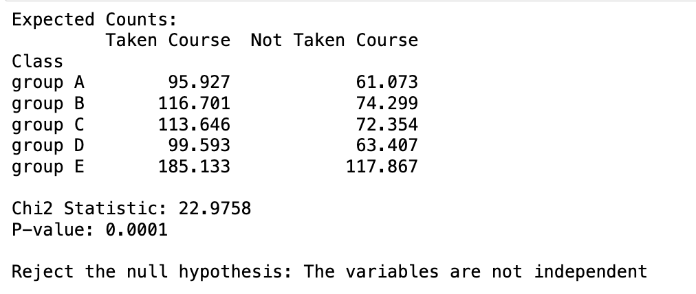
The rule of thumb is the same as the goodness-of-fit test: If our test statistic is more significant than the chi-squared table value we look up, we reject the null hypothesis. We will use the significance level of 5%. Because the total row is 5 and the total column is 2, we look up the value of chi-squared with a 5% significance level and degrees of freedom of (5–1) * (2–1) = 4, and we get 15.5. Because the test statistic is lower than the chi-squared table value (22.9758 > 15.5), we reject the null hypothesis at a 5% significance level.

Python Approach

This is the Python approach to the chi-squared contingency table test using SciPy:

import pandas as pd
from scipy.stats import chi2_contingency

# Create the dataset
data = {
    'Class': ['group A', 'group B', 'group C', 'group D', 'group E'],
    'Taken Course': [91, 131, 117, 75, 197],
    'Not Taken Course': [66, 60, 69, 88, 106]
}

# Create a DataFrame
df = pd.DataFrame(data)
df.set_index('Class', inplace=True)

# Perform the Chi-Squared test for independence
chi2_stat, p_val, dof, expected = chi2_contingency(df)

# Print the results
print("Expected Counts:")
print(pd.DataFrame(expected, index=df.index, columns=df.columns))
print(f"nChi2 Statistic: {chi2_stat:.4f}")
print(f"P-value: {p_val:.4f}")

# Print the conclusion
if p_val < 0.05:
    print("nReject the null hypothesis: The variables are not independent")
else:
    print("nFail to reject the null hypothesis: The variables are independent")

Using the p-value, we also got the same result. We reject the null hypothesis at a 5% significance level.

Now that you understand how to conduct hypothesis tests using the chi-square test method, it’s time to apply this knowledge to your own data. Happy experimenting!

Part 4: Conclusion

The chi-squared test is a powerful statistical method that helps us understand the relationships and distributions within categorical data. Forming the problem and proper hypotheses before jumping into the test itself is crucial. A large sample is also vital in conducting a chi-squared test; for instance, it works well for sizes down to 5,000 (Bergh, 2015), as small sample sizes can lead to inaccurate results. To interpret results correctly, choose the right significance level and compare the chi-square statistic to the critical value from the chi-square distribution table or the p-value.

Reference

• G. Keller, Statistics for Management and Economics, 11th ed., Chapter 15, Cengage Learning (2017).
• Daniel, Bergh. (2015). Chi-Squared Test of Fit and Sample Size-A Comparison between a Random Sample Approach and a Chi-Square Value Adjustment Method.. Journal of applied measurement, 16(2):204–217.

Chi-Squared Test: Revealing Hidden Patterns in Your Data was originally published in Towards Data Science on Medium, where people are continuing the conversation by highlighting and responding to this story.