LG is bringing a lamp that doubles as a small garden to CES 2025. The “indoor gardening appliance” is designed for apartment dwellers or anyone whose otherwise backyard-challenged to enjoy the benefits of homegrown produce.
During the day, LG says the lamp with a circular lampshade shines LEDs in five different intensities on whichever plants you want to grow. Then, at night, the lights fire upwards to create cozy mood lighting in whatever room you put the lamp in. If you’d prefer something that’s more compact and armchair-height, LG also has a version that the size of a side table.
LG
The taller, standing lamp can hold up to 20 plants at a time, according to LG, and the whole setup is height adjustable so that you can accommodate larger leafy greens or small herbs and flowers. The real beauty of LG’s design, though, is that you don’t need to worry about watering. There’s a 1.5 gallon tank built in to the base of the lamp that can disperse the appropriate amount of liquid for whatever you have planted. Both lamps are also connected to LG’s ThinQ app so you can adjust lighting and watering schedules remotely.
LG introduced its previous take on an indoor gardening tool, the LG Tiiun, at CES 2022. That larger, fridge-shaped appliance could also automatically grow and water plants, but was far less aesthetically-pleasing than the company’s new lamp. With all of the features it has on board, LG’s new lamp is really just one Sonos speaker away from being the ultimate living room appliance. At least until tech companies find another use for lamps.
LG’s new indoor gardening appliance doesn’t have a release date or an official price, but expect the company to share more details once CES 2025 officially starts.
This article originally appeared on Engadget at https://www.engadget.com/home/smart-home/lg-found-a-new-job-for-your-standing-lamp-173446654.html?src=rss
Understanding loss functions for training neural networks
Machine learning is very hands-on, and everyone charts their own path. There isn’t a standard set of courses to follow, as was traditionally the case. There’s no ‘Machine Learning 101,’ so to speak. However, this sometimes leaves gaps in understanding. If you’re like me, these gaps can feel uncomfortable. For instance, I used to be bothered by things we do casually, like the choice of a loss function. I admit that some practices are learned through heuristics and experience, but most concepts are rooted in solid mathematical foundations. Of course, not everyone has the time or motivation to dive deeply into those foundations — unless you’re a researcher.
I have attempted to present some basic ideas on how to approach a machine learning problem. Understanding this background will help practitioners feel more confident in their design choices. The concepts I covered include:
Quantifying the difference in probability distributions using cross-entropy.
A probabilistic view of neural network models.
Deriving and understanding the loss functions for different applications.
Entropy
In information theory, entropy is a measure of the uncertainty associated with the values of a random variable. In other words, it is used to quantify the spread of distribution. The narrower the distribution the lower the entropy and vice versa. Mathematically, entropy of distribution p(x) is defined as;
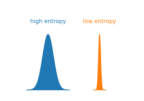
It is common to use log with the base 2 and in that case entropy is measured in bits. The figure below compares two distributions: the blue one with high entropy and the orange one with low entropy.
Visualization examples of distributions having high and low entropy — created by the author using Python.
We can also measure entropy between two distributions. For example, consider the case where we have observed some data having the distribution p(x) and a distribution q(x) that could potentially serve as a model for the observed data. In that case we can compute cross-entropy Hpq(X) between data distribution p(x) and the model distribution q(x). Mathematically cross-entropy is written as follows:
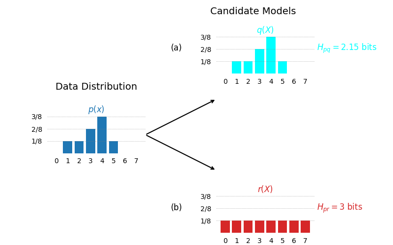
Using cross entropy we can compare different models and the one with lowest cross entropy is better fit to the data. This is depicted in the contrived example in the following figure. We have two candidate models and we want to decide which one is better model for the observed data. As we can see the model whose distribution exactly matches that of the data has lower cross entropy than the model that is slightly off.
Comparison of cross entropy of data distribution p(x) with two candidate models. (a) candidate model exactly matches data distribution and has low cross entropy. (b) candidate model does not match the data distribution hence it has high cross entropy — created by the author using Python.
There is another way to state the same thing. As the model distribution deviates from the data distribution cross entropy increases. While trying to fit a model to the data i.e. training a machine learning model, we are interested in minimizing this deviation. This increase in cross entropy due to deviation from the data distribution is defined as relative entropy commonly known as Kullback-Leibler Divergence of simply KL-Divergence.
Hence, we can quantify the divergence between two probability distributions using cross-entropy or KL-Divergence. To train a model we can adjust the parameters of the model such that they minimize the cross-entropy or KL-Divergence. Note that minimizing cross-entropy or KL-Divergence achieves the same solution. KL-Divergence has a better interpretation as its minimum is zero, that will be the case when the model exactly matches the data.
Another important consideration is how do we pick the model distribution? This is dictated by two things: the problem we are trying to solve and our preferred approach to solving the problem. Let’s take the example of a classification problem where we have (X, Y) pairs of data, with X representing the input features and Y representing the true class labels. We want to train a model to correctly classify the inputs. There are two ways we can approach this problem.
Discriminative vs Generative
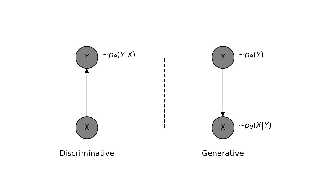
The generative approach refers to modeling the joint distribution p(X,Y) such that it learns the data-generating process, hence the name ‘generative’. In the example under discussion, the model learns the prior distribution of class labels p(Y) and for given class label Y, it learns to generate features X using p(X|Y).
It should be clear that the learned model is capable of generating new data (X,Y). However, what might be less obvious is that it can also be used to classify the given features X using Bayes’ Rule, though this may not always be feasible depending on the model’s complexity. Suffice it to say that using this for a task like classification might not be a good idea, so we should instead take the direct approach.
Discriminative vs generative approach of modelling — created by the author using Python.
Discriminative approach refers to modelling the relationship between input features X and output labels Y directly i.e. modelling the conditional distribution p(Y|X). The model thus learnt need not capture the details of features X but only the class discriminatory aspects of it. As we saw earlier, it is possible to learn the parameters of the model by minimizing the cross-entropy between observed data and model distribution. The cross-entropy for a discriminative model can be written as:
Where the right most sum is the sample average and it approximates the expectation w.r.t data distribution. Since our learning rule is to minimize the cross-entropy, we can call it our general loss function.
Goal of learning (training the model) is to minimize this loss function. Mathematically, we can write the same statement as follows:
Let’s now consider specific examples of discriminative models and apply the general loss function to each example.
Binary Classification
As the name suggests, the class label Y for this kind of problem is either 0 or 1. That could be the case for a face detector, or a cat vs dog classifier or a model that predicts the presence or absence of a disease. How do we model a binary random variable? That’s right — it’s a Bernoulli random variable. The probability distribution for a Bernoulli variable can be written as follows:
where π is the probability of getting 1 i.e. p(Y=1) = π.
Since we want to model p(Y|X), let’s make π a function of X i.e. output of our model π(X) depends on input features X. In other words, our model takes in features X and predicts the probability of Y=1. Please note that in order to get a valid probability at the output of the model, it has to be constrained to be a number between 0 and 1. This is achieved by applying a sigmoid non-linearity at the output.
To simplify, let’s rewrite this explicitly in terms of true label and predicted label as follows:
We can write the general loss function for this specific conditional distribution as follows:
This is the commonly referred to as binary cross entropy (BCE) loss.
Multi-class Classification
For a multi-class problem, the goal is to predict a category from C classes for each input feature X.In this case we can model the output Y as a categorical random variable, a random variable that takes on a state c out of all possible C states. As an example of categorical random variable, think of a six-faced die that can take on one of six possible states with each roll.
We can see the above expression as easy extension of the case of binary random variable to a random variable having multiple categories. We can model the conditional distribution p(Y|X) by making λ’s as function of input features X. Based on this, let’s we write the conditional categorical distribution of Y in terms of predicted probabilities as follows:
Using this conditional model distribution we can write the loss function using the general loss function derived earlier in terms of cross-entropy as follows:
This is referred to as Cross-Entropy loss in PyTorch. The thing to note here is that I have written this in terms of predicted probability of each class. In order to have a valid probability distribution over all C classes, a softmax non-linearity is applied at the output of the model. Softmax function is written as follows:
Regression
Consider the case of data (X, Y) where X represents the input features and Y represents output that can take on any real number value. Since Y is real valued, we can model the its distribution using a Gaussian distribution.
Again, since we are interested in modelling the conditional distribution p(Y|X). We can capture the dependence on X by making the conditional mean of Y a function of X. For simplicity, we set variance equal to 1. The conditional distribution can be written as follows:
We can now write our general loss function for this conditional model distribution as follows:
This is the famous MSE loss for training the regression model. Note that the constant factor is irrelevant here as we are only interest in finding the location of minima and can be dropped.
Summary
In this short article, I introduced the concepts of entropy, cross-entropy, and KL-Divergence. These concepts are essential for computing similarities (or divergences) between distributions. By using these ideas, along with a probabilistic interpretation of the model, we can define the general loss function, also referred to as the objective function. Training the model, or ‘learning,’ then boils down to minimizing the loss with respect to the model’s parameters. This optimization is typically carried out using gradient descent, which is mostly handled by deep learning frameworks like PyTorch. Hope this helps — happy learning!
Breaking the quadratic barrier: modern alternatives to softmax attention
Large Languange Models are great but they have a slight drawback that they use softmax attention which can be computationally intensive. In this article we will explore if there is a way we can replace the softmax somehow to achieve linear time complexity.
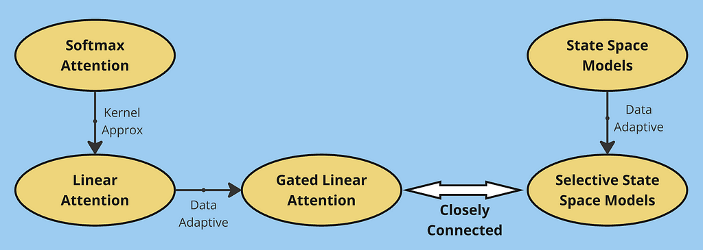
Image by Author (Created using Miro Board)
Attention Basics
I am gonna assume you already know about stuff like ChatGPT, Claude, and how transformers work in these models. Well attention is the backbone of such models. If we think of normal RNNs, we encode all past states in some hidden state and then use that hidden state along with new query to get our output. A clear drawback here is that well you can’t store everything in just a small hidden state. This is where attention helps, imagine for each new query you could find the most relevant past data and use that to make your prediction. That is essentially what attention does.
Attention mechanism in transformers (the architecture behind most current language models) involve key, query and values embeddings. The attention mechanism in transformers works by matching queries against keys to retrieve relevant values. For each query(Q), the model computes similarity scores with all available keys(K), then uses these scores to create a weighted combination of the corresponding values(Y). This attention calculation can be expressed as:
Source: Image by Author
This mechanism enables the model to selectively retrieve and utilize information from its entire context when making predictions. We use softmax here since it effectively converts raw similarity scores into normalized probabilities, acting similar to a k-nearest neighbor mechanism where higher attention weights are assigned to more relevant keys.
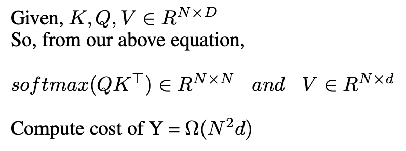
Okay now let’s see the computational cost of 1 attention layer,
Source: Image by Author
Softmax Drawback
From above, we can see that we need to compute softmax for an NxN matrix, and thus, our computation cost becomes quadratic in sequence length. This is fine for shorter sequences, but it becomes extremely computationally inefficient for long sequences, N=100k+.
This gives us our motivation: can we reduce this computational cost? This is where linear attention comes in.
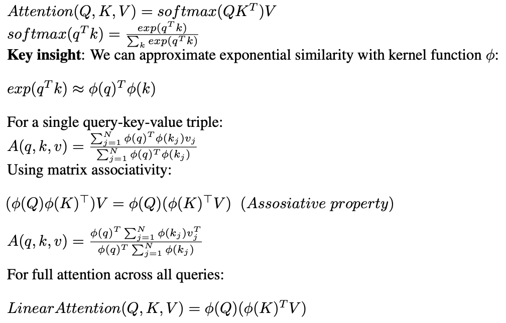
Linear Attention
Introduced by Katharopoulos et al., linear attention uses a clever trick where we write the softmax exponential as a kernel function, expressed as dot products of feature maps φ(x). Using the associative property of matrix multiplication, we can then rewrite the attention computation to be linear. The image below illustrates this transformation:
Source: Image by Author
Katharopoulos et al. used elu(x) + 1 as φ(x), but any kernel feature map that can effectively approximate the exponential similarity can be used. The computational cost of above can be written as,
Source: Image by Author
This eliminates the need to compute the full N×N attention matrix and reduces complexity to O(Nd²). Where d is the embedding dimension and this in effect is linear complexity when N >>> d, which is usually the case with Large Language Models
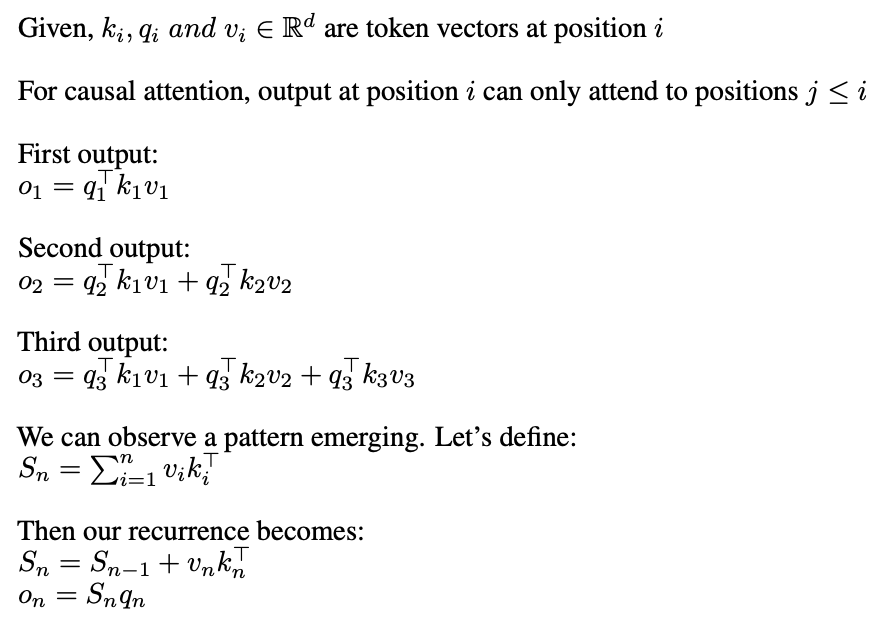
Okay let’s look at the recurrent view of linear attention,
Source: Image by Author
Okay why can we do this in linear attention and not in softmax? Well softmax is not seperable so we can’t really write it as product of seperate terms. A nice thing to note here is that during decoding, we only need to keep track of S_(n-1), giving us O(d²) complexity per token generation since S is a d × d matrix.
However, this efficiency comes with an important drawback. Since S_(n-1) can only store d² information (being a d × d matrix), we face a fundamental limitation. For instance, if your original context length requires storing 20d² worth of information, you’ll essentially lose 19d² worth of information in the compression. This illustrates the core memory-efficiency tradeoff in linear attention: we gain computational efficiency by maintaining only a fixed-size state matrix, but this same fixed size limits how much context information we can preserve and this gives us the motivation for gating.
Gated Linear Attention
Okay, so we’ve established that we’ll inevitably forget information when optimizing for efficiency with a fixed-size state matrix. This raises an important question: can we be smart about what we remember? This is where gating comes in — researchers use it as a mechanism to selectively retain important information, trying to minimize the impact of memory loss by being strategic about what information to keep in our limited state. Gating isn’t a new concept and has been widely used in architectures like LSTM
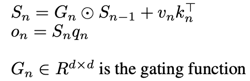
The basic change here is in the way we formulate Sn,
Source: Image by author
There are many choices for G all which lead to different models,
A key advantage of this architecture is that the gating function depends only on the current token x and learnable parameters, rather than on the entire sequence history. Since each token’s gating computation is independent, this allows for efficient parallel processing during training — all gating computations across the sequence can be performed simultaneously.
State Space Models
When we think about processing sequences like text or time series, our minds usually jump to attention mechanisms or RNNs. But what if we took a completely different approach? Instead of treating sequences as, well, sequences, what if we processed them more like how CNNs handle images using convolutions?
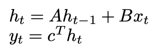
State Space Models (SSMs) formalize this approach through a discrete linear time-invariant system:
Source: Image by Author
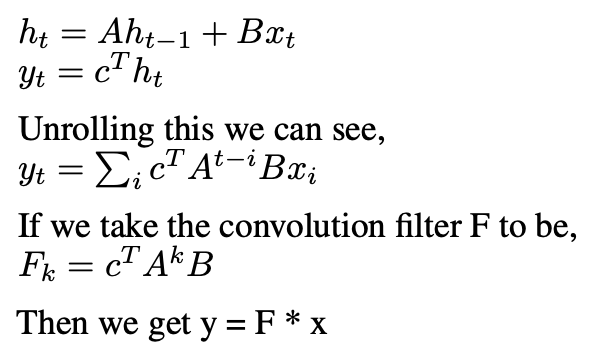
Okay now let’s see how this relates to convolution,
Source: Image by Author
where F is our learned filter derived from parameters (A, B, c), and * denotes convolution.
H3 implements this state space formulation through a novel structured architecture consisting of two complementary SSM layers.
Here we take the input and break it into 3 channels to imitate K, Q and V. We then use 2 SSM and 2 gating to kind of imitate linear attention and it turns out that this kind of architecture works pretty well in practice.
Selective State Space Models
Earlier, we saw how gated linear attention improved upon standard linear attention by making the information retention process data-dependent. A similar limitation exists in State Space Models — the parameters A, B, and c that govern state transitions and outputs are fixed and data-independent. This means every input is processed through the same static system, regardless of its importance or context.
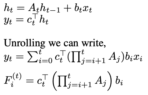
we can extend SSMs by making them data-dependent through time-varying dynamical systems:
Source: Image by Author
The key question becomes how to parametrize c_t, b_t, and A_t to be functions of the input. Different parameterizations can lead to architectures that approximate either linear or gated attention mechanisms.
Mamba implements this time-varying state space formulation through selective SSM blocks.
Mamba here uses Selective SSM instead of SSM and uses output gating and additional convolution to improve performance. This is a very high-level idea explaining how Mamba combines these components into an efficient architecture for sequence modeling.
Conclusion
In this article, we explored the evolution of efficient sequence modeling architectures. Starting with traditional softmax attention, we identified its quadratic complexity limitation, which led to the development of linear attention. By rewriting attention using kernel functions, linear attention achieved O(Nd²) complexity but faced memory limitations due to its fixed-size state matrix.
This limitation motivated gated linear attention, which introduced selective information retention through gating mechanisms. We then explored an alternative perspective through State Space Models, showing how they process sequences using convolution-like operations. The progression from basic SSMs to time-varying systems and finally to selective SSMs parallels our journey from linear to gated attention — in both cases, making the models more adaptive to input data proved crucial for performance.
Through these developments, we see a common theme: the fundamental trade-off between computational efficiency and memory capacity. Softmax attention excels at in-context learning by maintaining full attention over the entire sequence, but at the cost of quadratic complexity. Linear variants (including SSMs) achieve efficient computation through fixed-size state representations, but this same optimization limits their ability to maintain detailed memory of past context. This trade-off continues to be a central challenge in sequence modeling, driving the search for architectures that can better balance these competing demands.
To read more on this topics, i would suggest the following papers:
This blog post was inspired by coursework from my graduate studies during Fall 2024 at University of Michigan. While the courses provided the foundational knowledge and motivation to explore these topics, any errors or misinterpretations in this article are entirely my own. This represents my personal understanding and exploration of the material.
Linearizing Attention was originally published in Towards Data Science on Medium, where people are continuing the conversation by highlighting and responding to this story.
Reinforcement Learning (RL) is a branch of Artificial Intelligence that enables agents to learn how to interact with their environment. These agents, which range from robots to software features or autonomous systems, learn through trial and error. They receive rewards or penalties based on the actions they take, which guide their future decisions.
Among the most well-known RL algorithms, Proximal Policy Optimization (PPO) is often favored for its stability and efficiency. PPO addresses several challenges in RL, particularly in controlling how the policy (the agent’s decision-making strategy) evolves. Unlike other algorithms, PPO ensures that policy updates are not too large, preventing destabilization during training. This stabilization is crucial, as drastic updates can cause the agent to diverge from an optimal solution, making the learning process erratic. PPO thus maintains a balance between exploration (trying new actions) and exploitation (focusing on actions that yield the highest rewards).
Additionally, PPO is highly efficient in terms of both computational resources and learning speed. By optimizing the agent’s policy effectively while avoiding overly complex calculations, PPO has become a practical solution in various domains, such as robotics, gaming, and autonomous systems. Its simplicity makes it easy to implement, which has led to its widespread adoption in both research and industry.
This article explores the mathematical foundations of RL and the key concepts introduced by PPO, providing a deeper understanding of why PPO has become a go-to algorithm in modern reinforcement learning research.
1. The Basics of RL: Markov Decision Process (MDP)
Reinforcement learning problems are often modeled using a Markov Decision Process (MDP), a mathematical framework that helps formalize decision-making in environments where outcomes are uncertain.
A Markov chain models a system that transitions between states, where the probability of moving to a new state depends solely on the current state and not on previous states. This principle is known as the Markov property. In the context of MDPs, this simplification is key for modeling decisions, as it allows an agent to focus only on the current state when making decisions without needing to account for the entire history of the system.
An MDP is defined by the following elements: – S: Set of possible states. – A: Set of possible actions. – P(s’|s, a): Transition probability of reaching state s’ after taking action a in state s. – R(s, a): Reward received after taking action a in state s. – γ: Discount factor (a value between 0 and 1) that reflects the importance of future rewards.
The discount factor γ is crucial for modeling the importance of future rewards in decision-making problems. When an agent makes a decision, it must evaluate not only the immediate reward but also the potential future rewards. The discount γ reduces the impact of rewards that occur later in time due to the uncertainty of reaching those rewards. Thus, a value of γ close to 1 indicates that future rewards are almost as important as immediate rewards, while a value close to 0 gives more importance to immediate rewards.
The time discount reflects the agent’s preference for quick gains over future ones, often due to uncertainty or the possibility of changes in the environment. For example, an agent will likely prefer an immediate reward rather than one in the distant future unless that future reward is sufficiently significant. This discount factor thus models optimization behaviors where the agent considers both short-term and long-term benefits.
The goal is to find an action policy π(a|s) that maximizes the expected sum of rewards over time, often referred to as the value function:
This function represents the expected total reward an agent can accumulate starting from state s and following policy π.
2. Policy Optimization: Policy Gradient
Policy gradient methods focus on directly optimizing the parameters θ of a policy πθ by maximizing an objective function that represents the expected reward obtained by following that policy in a given environment.
The objective function is defined as:
Where R(s, a) is the reward received for taking action a in state s, and the goal is to maximize this expected reward over time. The term dπ(s) represents the stationary distribution of states under policy π, indicating how frequently the agent visits each state when following policy π.
The policy gradient theorem gives the gradient of the objective function, providing a way to update the policy parameters:
This equation shows how to adjust the policy parameters based on past experiences, which helps the agent learn more efficient behaviors over time.
3. Mathematical Enhancements of PPO
PPO (Proximal Policy Optimization) introduces several important features to improve the stability and efficiency of reinforcement learning, particularly in large and complex environments. PPO was introduced by John Schulman et al. in 2017 as an improvement over earlier policy optimization algorithms like Trust Region Policy Optimization (TRPO). The main motivation behind PPO was to strike a balance between sample efficiency, ease of implementation, and stability while avoiding the complexities of TRPO’s second-order optimization methods. While TRPO ensures stable policy updates by enforcing a strict constraint on the policy change, it relies on computationally expensive second-order derivatives and conjugate gradient methods, making it challenging to implement and scale. Moreover, the strict constraints in TRPO can sometimes overly limit policy updates, leading to slower convergence. PPO addresses these issues by using a simple clipped objective function that allows the policy to update in a stable and controlled manner, avoiding forgetting previous policies with each update, thus improving training efficiency and reducing the risk of policy collapse. This makes PPO a popular choice for a wide range of reinforcement learning tasks.
a. Probability Ratio
One of the key components of PPO is the probability ratio, which compares the probability of taking an action in the current policy πθ to that of the old policy πθold:
This ratio provides a measure of how much the policy has changed between updates. By monitoring this ratio, PPO ensures that updates are not too drastic, which helps prevent instability in the learning process.
b. Clipping Function
Clipping is preferred over adjusting the learning rate in Proximal Policy Optimization (PPO) because it directly limits the magnitude of policy updates, preventing excessive changes that could destabilize the learning process. While the learning rate uniformly scales the size of updates, clipping ensures that updates stay close to the previous policy, thereby enhancing stability and reducing erratic behavior.
The main advantage of clipping is that it allows for better control over updates, ensuring more stable progress. However, a potential drawback is that it may slow down learning by limiting the exploration of significantly different strategies. Nonetheless, clipping is favored in PPO and other algorithms when stability is essential.
To avoid excessive changes to the policy, PPO uses a clipping function that modifies the objective function to restrict the size of policy updates. This is crucial because large updates in reinforcement learning can lead to erratic behavior. The modified objective with clipping is:
The clipping function constrains the probability ratio within a specific range, preventing updates that would deviate too far from the previous policy. This helps avoid sudden, large changes that could destabilize the learning process.
c. Advantage Estimation with GAE
In RL, estimating the advantage is important because it helps the agent determine which actions are better than others in each state. However, there is a trade-off: using only immediate rewards (or very short horizons) can introduce high variance in advantage estimates, while using longer horizons can introduce bias.
Generalized Advantage Estimation (GAE) strikes a balance between these two by using a weighted average of n-step returns and value estimates, making it less sensitive to noise and improving learning stability.
Why use GAE? – Stability: GAE helps reduce variance by considering multiple steps so the agent does not react to noise in the rewards or temporary fluctuations in the environment. – Efficiency: GAE strikes a good balance between bias and variance, making learning more efficient by not requiring overly long sequences of rewards while still maintaining reliable estimates. – Better Action Comparison: By considering not just the immediate reward but a broader horizon of rewards, the agent can better compare actions over time and make more informed decisions.
The advantage function At is used to assess how good an action was relative to the expected behavior under the current policy. To reduce variance and ensure more reliable estimates, PPO uses Generalized Advantage Estimation (GAE). This method smooths out the advantages over time while controlling for bias:
This technique provides a more stable and accurate measure of the advantage, which improves the agent’s ability to make better decisions.
d. Entropy to Encourage Exploration
PPO incorporates an entropy term in the objective function to encourage the agent to explore more of the environment rather than prematurely converging to a suboptimal solution. The entropy term increases the uncertainty in the agent’s decision-making, which prevents overfitting to a specific strategy:
Where H(πθ) represents the entropy of the policy. By adding this term, PPO ensures that the agent does not converge too quickly and is encouraged to continue exploring different actions and strategies, improving overall learning efficiency.
Conclusion
The mathematical underpinnings of PPO demonstrate how this algorithm achieves stable and efficient learning. With concepts like the probability ratio, clipping, advantage estimation, and entropy, PPO offers a powerful balance between exploration and exploitation. These features make it a robust choice for both researchers and practitioners working in complex environments. The simplicity of PPO, combined with its efficiency and effectiveness, makes it a popular and valuable algorithm in reinforcement learning.
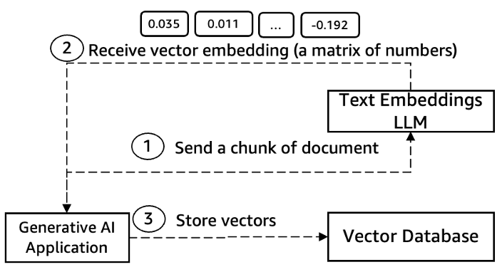
Optimizing costs of generative AI applications on AWS is critical for realizing the full potential of this transformative technology. The post outlines key cost optimization pillars, including model selection and customization, token usage, inference pricing plans, and vector database considerations.
We use cookies on our website to give you the most relevant experience by remembering your preferences and repeat visits. By clicking “Accept”, you consent to the use of ALL the cookies.
This website uses cookies to improve your experience while you navigate through the website. Out of these, the cookies that are categorized as necessary are stored on your browser as they are essential for the working of basic functionalities of the website. We also use third-party cookies that help us analyze and understand how you use this website. These cookies will be stored in your browser only with your consent. You also have the option to opt-out of these cookies. But opting out of some of these cookies may affect your browsing experience.
Necessary cookies are absolutely essential for the website to function properly. These cookies ensure basic functionalities and security features of the website, anonymously.
Cookie
Duration
Description
cookielawinfo-checkbox-analytics
11 months
This cookie is set by GDPR Cookie Consent plugin. The cookie is used to store the user consent for the cookies in the category "Analytics".
cookielawinfo-checkbox-functional
11 months
The cookie is set by GDPR cookie consent to record the user consent for the cookies in the category "Functional".
cookielawinfo-checkbox-necessary
11 months
This cookie is set by GDPR Cookie Consent plugin. The cookies is used to store the user consent for the cookies in the category "Necessary".
cookielawinfo-checkbox-others
11 months
This cookie is set by GDPR Cookie Consent plugin. The cookie is used to store the user consent for the cookies in the category "Other.
cookielawinfo-checkbox-performance
11 months
This cookie is set by GDPR Cookie Consent plugin. The cookie is used to store the user consent for the cookies in the category "Performance".
viewed_cookie_policy
11 months
The cookie is set by the GDPR Cookie Consent plugin and is used to store whether or not user has consented to the use of cookies. It does not store any personal data.
Functional cookies help to perform certain functionalities like sharing the content of the website on social media platforms, collect feedbacks, and other third-party features.
Performance cookies are used to understand and analyze the key performance indexes of the website which helps in delivering a better user experience for the visitors.
Analytical cookies are used to understand how visitors interact with the website. These cookies help provide information on metrics the number of visitors, bounce rate, traffic source, etc.
Advertisement cookies are used to provide visitors with relevant ads and marketing campaigns. These cookies track visitors across websites and collect information to provide customized ads.