A discussion around measuring error rates in IBM quantum processors, with code examples, using Qiskit
Quantum computing has made significant strides in recent years, with breakthroughs in hardware stability, error mitigation, and algorithm development bringing us closer to solving problems that classical computers cannot tackle efficiently. Companies and research institutions worldwide are pushing the boundaries of what quantum systems can achieve, transforming this once-theoretical field into a rapidly evolving technology. IBM has emerged as a key player in this space, offering IBM Quantum, a platform that provides access to state-of-the-art quantum processors (QPUs) with a qubit capacity in the hundreds. Through the open-source Qiskit SDK, developers, researchers, and enthusiasts can design, simulate, and execute quantum circuits on real quantum hardware. This accessibility has accelerated innovation while also highlighting key challenges, such as managing the error rates that still limit the performance of today’s quantum devices.
By leveraging the access to quantum processors available for free on the IBM platform, we propose to run a few quantum computations to measure the current level of quantum noise in basic circuits. Achieving a low enough level of quantum noise is the most important challenge in making quantum computing useful. Unfortunately, there is not a ton of material on the web explaining the current achievements. It is also not obvious what quantity we want to measure and how to measure it in practice.
In this blogpost,
- We will review some basics of quantum circuits manipulations in Qiskit.
- We will explain the minimal formalism to discuss quantum errors, explaining the notion of quantum state fidelity.
- We will show how to estimate the fidelity of states produced by simple quantum circuits.
To follow this discussion, you will need to know some basics about Quantum Information Theory, namely what are qubits, gates, measurements and, ideally, density matrices. The IBM Quantum Learning platform has great free courses to learn the basics and more on this topic.
Disclaimer: Although I am aiming at a decent level of scientific rigorousness, this is not a research paper and I do not pretend to be an expert in the field, but simply an enthusiast, sharing my modest understanding.
To start with, we need to install Qiskit tools
%pip install qiskit qiskit_ibm_runtime
%pip install 'qiskit[visualization]'
import qiskit
import qiskit_ibm_runtime

print(qiskit.version.get_version_info())
print(qiskit_ibm_runtime.version.get_version_info())
1.3.1
0.34.0
Running a quantum circuit and observing errors
Quantum computations consist in building quantum circuits, running them on quantum hardware and collecting the measured outputs.
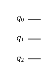
To build a quantum circuit, we start by specifying a number n of qubits for our circuits, where n can be as large as 127 or 156, depending on the underling QPU instance (see processor types). All n qubits are initialised in the |0⟩ state, so the initial state is |0 ⟩ⁿ . Here is how we initialise a circuit with 3 qubits in Qiskit.
from qiskit.circuit import QuantumCircuit

# A quantum circuit with three qubits
qc = QuantumCircuit(3)
qc.draw('mpl')
Next we can add operations on those qubits, in the form of quantum gates, which are unitary operations acting typically on one or two qubits. For instance let us add one Hadamard gate acting on the first qubit and two CX (aka CNOT) gates on the pairs of qubits (0, 1) and (0, 2).
# Hadamard gate on qubit 0.
qc.h(0)
# CX gates on qubits (0, 1) and (0, 2).
qc.cx(0, 1)
qc.cx(0, 2)

qc.draw('mpl')
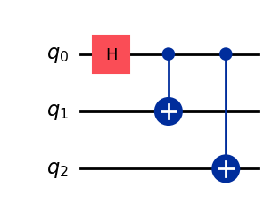
We obtain a 3-qubit circuit preparing the state

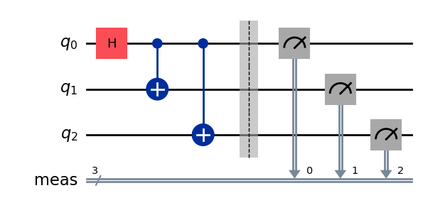
To measure the output qubits of the circuit, we add a measurement layer
qc.measure_all()
qc.draw('mpl')
It is possible to run the circuit and to get its output measured bits as a simulation with StatevectorSampleror on real quantum hardware with SamplerV2 . Let us see the output of a simulation first.
from qiskit.primitives import StatevectorSampler
from qiskit.transpiler.preset_passmanagers import generate_preset_pass_manager
from qiskit.visualization import plot_distribution

sampler = StatevectorSampler()
pm = generate_preset_pass_manager(optimization_level=1)
# Generate the ISA circuit
qc_isa = pm.run(qc)
# Run the simulator 10_000 times
num_shots = 10_000
result = sampler.run([qc_isa], shots=num_shots).result()[0]
# Collect and plot measurements
measurements= result.data.meas.get_counts()
plot_distribution(measurements)
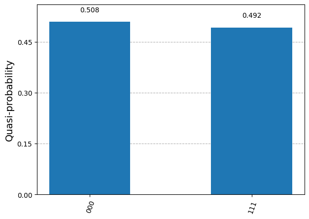
The measured bits are either (0,0,0) or (1,1,1), with approximate probability close to 0.5. This is precisely what we expect from sampling the 3-qubit state prepared by the circuit.
We now run the circuit on a QPU (see instructions on setting up an IBM Quantum account and retrieving your personal token)
from qiskit_ibm_runtime import QiskitRuntimeService
from qiskit_ibm_runtime import SamplerV2 as Sampler

service = QiskitRuntimeService(
    channel="ibm_quantum",
    token=<YOUR_TOKEN>, # use your IBM Quantum token here.
)
# Fetch a QPU to use
backend = service.least_busy(operational=True, simulator=False)
print(f"QPU: {backend.name}")
target = backend.target
sampler = Sampler(mode=backend)
pm = generate_preset_pass_manager(target=target, optimization_level=1)
# Generate the ISA circuit
qc_isa = pm.run(qc)
# Run the simulator 10_000 times
num_shots = 10_000
result = sampler.run([qc_isa], shots=num_shots).result()[0]
# Collect and plot measurements
measurements= result.data.meas.get_counts()
plot_distribution(measurements)
QPU: ibm_brisbane
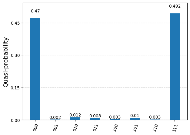
The measured bits are similar to those of the simulation, but now we see a few occurrences of the bit triplets (0,0,1), (0,1,0), (1,0,0), (0,1,1), (1,0,1) and (1,1,0). Those measurements should not occur from sampling the 3-qubit state prepared by the chosen circuit. They correspond to quantum errors occurring while running the circuit on the QPU.
We would like to quantify the error rate somehow, but it is not obvious how to do it. In quantum computations, what we really care about is that the qubit quantum state prepared by the circuit is the correct state. The measurements which are not (0,0,0) or (1,1,1) indicate errors in the state preparation, but this is not all. The measurements (0,0,0) and (1,1,1) could also be the result of incorrectly prepared states, e.g. the state (|0,0,0⟩ + |0,0,1⟩)/√2 can produce the output (0,0,0). Actually, it seems very likely that a few of the “correct” measurements come from incorrect 3-qubit states.
To understand this “noise” in the state preparation we need the formalism of density matrices to represent quantum states.
Density matrices and state fidelity
The state of an n-qubit circuit with incomplete information is represented by a 2ⁿ× 2ⁿ positive semi-definite hermitian matrix with trace equal to 1, called the density matrix ρ. Each diagonal element corresponds to the probability pᵢ of measuring one of the 2ⁿ possible states in a projective measurement, pᵢ = ⟨ψᵢ| ρ |ψᵢ⟩. The off-diagonal elements in ρ do not really have a physical interpretation, they can be set to zero by a change of basis states. In the computational basis, i.e. the standard basis |bit₀, bit₁, …, bitₙ⟩, they encode the entanglement properties of the state. Vector states |ψ⟩ describing the possible quantum states of the qubits have density matrices ρ = |ψ⟩⟨ψ|, whose eigenvalues are all 0, except for one eigenvalue, which is equal to 1. They are called pure states. Generic density matrices represent probabilistic quantum states of the circuit and have eigenvalues between 0 and 1. They are called mixed states. To give an example, a circuit which is in a state |ψ₁⟩ with probability q and in a state |ψ₂⟩ with probability 1-q is represented by the density matrix ρ = q|ψ₁⟩⟨ψ₁| + (1-q)|ψ₂⟩⟨ψ₂|.
In real quantum hardware, qubits are subject to all kinds of small unknown interactions with the environment, leading to a “loss of information”. This is the source of an incoherent quantum noise. Therefore, when applying gates to qubits or even when preparing the initial state, the quantum state of qubits cannot be described by a pure state, but ends up in a mixed state, which we must describe with a density matrix ρ. Density matrices provide a convenient way to describe quantum circuits in isolation, abstracting the complex and unknown interactions with the environment.
To learn more about density matrix representation of quantum states, you can look at any quantum information course. The excellent Qiskit lecture on this topic is available on YouTube.
For a single qubit, the density matrix, in the computational basis (i.e. the basis {|0⟩, |1⟩}), is a 2×2 matrix

with p₀ = ⟨0|ρ|0⟩ the probability to measure 0, p₁ = 1 — p₀ = ⟨1|ρ|1⟩ the probability to measure 1, and c is a complex number bounded by |c|² ≤ p₀p₁. Pure states have eigenvalues 0 and 1, so their determinant is zero, and they saturate the inequality with |c|² = p₀p₁.
In the following, we will consider quantum circuits with a few qubits and we will be interested in quantifying how close the output state density matrix ρ is from the expected (theoretical) output density matrix ρ₀. For a single qubit state, we could think about comparing the values of p₀, p₁ and c, provided we are able to measure them, but in a circuit with more qubits and a larger matrix ρ, we would like to come up with a single number quantifying how close ρ and ρ₀ are. Quantum information theory possesses such quantity. It is called state fidelity and it is defined by the slightly mysterious formula

The state fidelity F is a real number between 0 an 1, 0 ≤ F ≤ 1, with F = 1 corresponding to having identical states ρ = ρ₀ , and F = 0 corresponding to ρ and ρ₀ having orthogonal images. Although it is not so obvious from the definition, it is a symmetric quantity, F(ρ,ρ₀) = F(ρ₀,ρ).
In quantum circuit computations, the expected output state ρ₀ is always a pure state ρ₀ = |ψ₀⟩⟨ψ₀| and, in this case, the state fidelity reduces to the simpler formula

which has the desired interpretation as the probability for the state ρ to be measured in the state |ψ₀⟩ (in a hypothetical experiment implementing a projective measurement onto the state |ψ₀⟩ ).
In the noise-free case, the produced density matrix is ρ = ρ₀ = |ψ₀⟩⟨ψ₀| and the state fidelity is 1. In the presence of noise the fidelity decreases, F < 1.
In the remainder of this discussion, our goal will be to measure the state fidelity F of simple quantum circuit in Qiskit, or, more precisely, to estimate a lower bound F̃ < F.
State fidelity estimation in quantum circuits
To run quantum circuits on QPUs and collect measurement results, we define the function run_circuit .
def run_circuit(
        qc: QuantumCircuit,
        service: QiskitRuntimeService = service,
        num_shots: int = 100,
    ) -> tuple[dict[str, int], QuantumCircuit]:
    """Runs the circuit on backend 'num_shots' times. Returns the counts of
    measurements and the ISA circuit."""
    # Fetch an available QPU
    backend = service.least_busy(operational=True, simulator=False)
    target = backend.target
    pm = generate_preset_pass_manager(target=target, optimization_level=1)

    # Add qubit mesurement layer and compute ISA circuit
    qc_meas = qc.measure_all(inplace=False)
    qc_isa = pm.run(qc_meas)

    # Run the ISA circuit and collect results
    sampler = Sampler(mode=backend)
    result = sampler.run([qc_isa], shots=num_shots).result()
    dist = result[0].data.meas.get_counts()

    return dist, qc_isa
The ISA (Instruction Set Architecture) circuit qc_isa returned by this function is essentially a rewriting of the provided circuit in terms of the physical gates available on the QPU, called basis gates. This is the circuit that is actually constructed and run on the hardware.
Note: The run_circuit function starts by fetching an available QPU. This is convenient to avoid waiting too long for the computation to be processed. However this also means that we use different QPUs each time we call the function. This is not ideal, as it is possible that different QPUs have different level of quantum noise. However, in practice, the fetched QPUs all turned out to be in the Eagle family and we present noise estimation only for this QPU family. To keep our analysis simple, we just assume that the level of quantum noise among the possible QPU instances is stable. The interested reader could try to find whether there are differences between instances.
Bare |0⟩ state
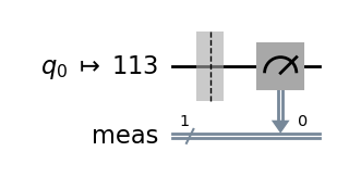
Let us start with the simplest circuit, which comprises only an initialised qubit |0⟩ without any gate operation.
# A quantum circuit with a single qubit |0>
qc = QuantumCircuit(1)
dist, qc_isa = run_circuit(qc, num_shots=100_000)
qc_isa.draw(output="mpl", idle_wires=False, style="iqp")
import numpy as np

def print_results(dist: dict[str, int]) -> None:
    print(f"Measurement counts: {dist}")
    num_shots = sum([dist[k] for k in dist])
    for k, v in dist.items():
        p = v / num_shots
        # 1% confidence interval estimate for a Bernoulli variable
        delta = 2.575 * np.sqrt(p*(1-p)/num_shots)
        print(f"p({k}): {np.round(p, 4)}  ± {np.round(delta, 4)}")

print_results(dist)
Measurement counts: {'0': 99661, '1': 339}
p(0) = 0.9966 ± 0.0005
p(1) = 0.0034 ± 0.0005
We get a small probability, around 0.3%, to observe the incorrect result 1. The interval estimate “± 0.0005” refers to a 1% confidence interval estimate for a Bernoulli variable.
The fidelity of the output state ρ, relative to the ideal state |0⟩, is F = ⟨0|ρ|0⟩ = p₀. We have obtained an estimate of 0.9966 ± 0.0005 for p₀ from the repeated measurements of the circuit output state. But the measurement operation is a priori imperfect (it has its own error rate). It may add a bias to the p₀ estimate. We assume that these measurement errors tend to decrease the estimated fidelity by incorrect measurements of |0⟩ states. In this case, the estimated p₀ will be a lower bound on the true fidelity F:
F > F̃ = 0.9966 ± 0.0005
Note: We have obtained estimated probabilities p₀, p₁ for the diagonal components of the single-qubit density matrix ρ. We also have an estimated bound on the off-diagonal component |c| < √(p₀ p₁) ~ 0.06. To get an actual estimate for c, we would need to run a circuit some gates and design a more complex reasoning.
Basis gates
Qiskit offers a large number of quantum gates encoding standard operations on one or two qubits, however all these gates are encoded in the QPU hardware with combinations of a very small set of physical operations on the qubits, called basis gates.
There are three single-qubit basis gates: X, SX and RZ(λ) and one two-qubit basis gate: ECR. All other quantum gates are constructed from these building blocks. The more basis gates are used in a quantum circuit, the larger is the quantum noise. We will analyse the noise resulting from applying these basis gates in isolation, when possible, or with a minimal number of basis gates, to get a sense of quantum noise in the current state of QPU computations.
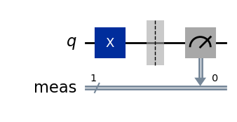
X gate
We consider the circuit made of a single qubit and an X gate. The output state, in the absence of noise, is X|0⟩ = |1⟩.
# Quantum circuit with a single qubit and an X gate.
# Expected output state X|0> = |1>.
qc = QuantumCircuit(1)
qc.x(0)

dist, qc_isa = run_circuit(qc, num_shots=100_000)
qc_isa.draw(output="mpl", idle_wires=False, style="iqp")
print_results(dist)
Measurement counts: {'1': 99072, '0': 928}
p(0) = 0.0093 ± 0.0008
p(1) = 0.9907 ± 0.0008
The state fidelity of the output state ρ, relative to the ideal state |1⟩, is
F = ⟨1|ρ|1⟩ = p₁ > F̃ = 0.9907 ± 0.0008
where we assumed again that the measurement operation lower the estimated fidelity and we get a lower bound F̃ on the fidelity.
We observe that the fidelity is (at least) around 99.1%, which is a little worse than the fidelity measured without the X gate. Indeed, adding a gate to the circuit should add noise, but there can be another effect contributing to the degradation of the fidelity, which is the fact that the |1⟩ state is a priori less stable than the |0⟩ state and so the measurement of a |1⟩ state itself is probably more noisy. We will not discuss the physical realisation of a qubit in IBM QPUs, but one thing to keep in mind is that the |0⟩ state has lower energy than the |1⟩ state, so that it is quantum mechanically more stable. As a result, the |1⟩ state can decay to the |0⟩ state through interactions with the environement.
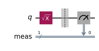
SX gate
We now consider the SX gate, i.e. the “square-root X” gate, represented by the matrix

It transforms the initial qubit state |0⟩ into the state

# Quantum circuit with a single qubit and an SX gate.
qc = QuantumCircuit(1)
qc.sx(0)

dist, qc_isa = run_circuit(qc, num_shots=100_000)
qc_isa.draw(output="mpl", idle_wires=False, style="iqp")
print_results(dist)
Measurement counts: {'1': 50324, '0': 49676}
p(0) = 0.4968 ± 0.0041
p(1) = 0.5032 ± 0.0041
We observe roughly equal distributions of zeros and ones, which is as expected. But we face a problem now. The state fidelity cannot be computed from these p₀ and p₁ estimates. Indeed, the fidelity of the output state ρ, relative to the ideal output state SX|0⟩ is

Therefore, to get an estimate of F, we also need to measure c, or rather its imaginary part Im(c). Since there is no other measurement we can do on the SX gate circuit, we need to consider a circuit with more gates to evaluate F, but more gates also means more sources of noise.
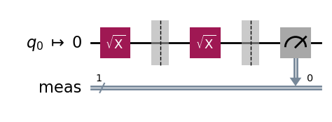
One simple thing we can do is to add either another SX gate or an SX⁻¹ gate. In the former case, the full circuit implements the X operation and the expected final state |1⟩, while in the latter case, the full circuit implements the identity operation and the expected final state is |0⟩.
Let us consider the case of adding an SX gate: the density matrix ρ produced by the first SX gate gets transformed into

leading to p’₁ = 1/2— Im(c) = F, in the ideal case when the second SX gate is free of quantum noise. In practice the SX gate is imperfect and we can only measure p’₁ = 1/2 — Im(c) — δp = F — δp, where δp is due to the noise from the second SX gate. Although it is theoretically possible that the added noise δp combines with the noise introduced by the first SX gate and results in a smaller combined noise, we will assume that no such “happy” cancelation happens, so that we have δp>0. In this case, p’₁ < F gives us a lower bound on the state fidelity F.
qc = QuantumCircuit(1)
qc.sx(0)
qc.barrier() # Prevents simplification of the circuit during transpilation.
qc.sx(0)

dist, qc_isa = run_circuit(qc, num_shots=100_000)
print_results(dist)
Measurement counts: {'1': 98911, '0': 1089}
p(1): 0.9891  ± 0.0008
p(0): 0.0109  ± 0.0008
We obtain a lower bound F > p’₁ = 0.9891 ± 0.0008, on the fidelity of the output state ρ for the SX-gate circuit, relative to the ideal output state SX|0⟩.
We could have considered the two-gate circuit with an SX gate followed by an SX⁻¹ gate instead. The SX⁻¹ gate is not a basis gate. It is implemented in the QPU as SX⁻¹ = RZ(-π) SX RZ(-π). We expect this setup to add more quantum noise due the presence of more basis gates, but in practice we have measured a higher (better) lower bound F̃. The interested reader can check this as an exercise. We believe this is due to the fact that the unwanted interactions with the environment tend to bring the qubit state to the ground state |0⟩, improving incorrectly the lower bound estimate, so we do not report this alternative result.
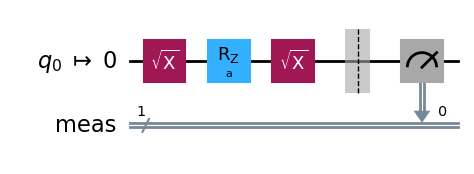
RZ(λ) gate
Next we consider the RZ(λ) gate. The RZ(λ) gate is a parametrised gate implementing a rotation around the z-axis by an angle λ/2.

Its effect on the initial qubit |0⟩ is only to multiply it by a phase exp(-iλ/2), leaving it in the same state. In general, the action of RZ(λ) on the density matrix of a single qubit is to multiply the off-diagonal coefficient c by exp(iλ), leaving the p₀ and p₁ values of the state unchanged. To measure a non-trivial effect of the RZ(λ) gate, one needs to consider circuits with more gates. The simplest is to consider the circuit composing the three gates SX, RZ(λ) and SX, preparing the state

The expected p(0) and p(1) values are

Qiskit offers the possibility to run parametrised quantum circuits by specifying an array of parameter values, which, together with the ISA circuit, define a Primitive Unified Bloc (PUB). The PUB is then passed to the sampler to run the circuit with all the specified parameter values.
from qiskit.primitives.containers.sampler_pub_result import SamplerPubResult

def run_parametrised_circuit(
        qc: QuantumCircuit,
        service: QiskitRuntimeService = service,
        params: np.ndarray | None = None,
        num_shots: int = 100,
    ) -> tuple[SamplerPubResult, QuantumCircuit]:
    """Runs the parametrised circuit on backend 'num_shots' times.
    Returns the PubResult and the ISA circuit."""
    # Fetch an available QPU
    backend = service.least_busy(operational=True, simulator=False)
    target = backend.target
    pm = generate_preset_pass_manager(target=target, optimization_level=1)

    # Add mesurement layer
    qc_meas = qc.measure_all(inplace=False)
    # Define ISA circuit and PUB
    pm = generate_preset_pass_manager(target=target, optimization_level=1)
    qc_isa = pm.run(qc_meas)
    sampler_pub = (qc_isa, params)

    # Run the circuit
    result = sampler.run([sampler_pub], shots=num_shots).result()
    return result[0], qc_isa
from qiskit.circuit import Parameter

# Circuit preparing the state SX.RZ(a).SX|0> = sin(a/2)|0> + cos(a/2)|1>.
qc = QuantumCircuit(1)
qc.sx(0)
qc.rz(Parameter("a"), 0)
qc.sx(0)

# Define parameter range
params = np.linspace(0, 2*np.pi, 21).reshape(-1, 1)
# Run parametrised circuit
pub_result, qc_isa = run_parametrised_circuit(qc, params=params, num_shots=10_000)

qc_isa.draw(output="mpl", idle_wires=False, style="iqp")
bit_array = pub_result.data.meas.bitcount()
print(f"bit_array shape: {bit_array.shape}")
p0 = (bit_array.shape[1] - bit_array.sum(axis=1)) / bit_array.shape[1]
p1 = bit_array.sum(axis=1) / bit_array.shape[1]
print(f"p(0): {p0}")
print(f"p(1): {p1}")
bit_array shape: (21, 10000)
p(0): [0.0031 0.0265 0.095  0.2095 0.3507 0.4969 0.6567 0.7853 0.9025 0.9703
 0.9983 0.976  0.901  0.7908 0.6543 0.5013 0.3504 0.2102 0.0982 0.0308
 0.0036]
p(1): [0.9969 0.9735 0.905  0.7905 0.6493 0.5031 0.3433 0.2147 0.0975 0.0297
 0.0017 0.024  0.099  0.2092 0.3457 0.4987 0.6496 0.7898 0.9018 0.9692
 0.9964]
import matplotlib.pyplot as plt

x = params/(2*np.pi)
plt.scatter(x, p0)
plt.scatter(x, p1)
plt.plot(x, np.sin(np.pi*x)**2, linestyle="--")
plt.plot(x, np.cos(np.pi*x)**2, linestyle="--")
plt.xlabel("λ/2π")
plt.ylabel("Estimated probabilities")
plt.legend(["p(0)", "p(1)", "sin(λ/2)^2", "cos(λ/2)^2"])
plt.show()

We see that the estimated probabilities (blue and orange dots) agree very well with the theoretical probabilities (blue and orange lines) for all tested values of λ.
Here again, this does not give us the state fidelity. We can give a lower bound by adding another sequence of gates SX.RZ(λ).SX to the circuit, bringing back the state to |0⟩. As in the case of the SX gate of the previous section, the estimated F̃ := p’₀ from this 6-gate circuit gives us a lower bound on the fidelity of the F of the 3-gate circuit, assuming the extra gates lower the output state fidelity.
Let us compute this lower bound F̃ for one value, λ = π/4.
# Circuit implementing SX.RZ(π/4).SX.SX.RZ(π/4).SX|0> = |0>
qc = QuantumCircuit(1)
qc.sx(0)
qc.rz(np.pi/4, 0)
qc.sx(0)
qc.barrier()  # Prevents circuit simplifications.
qc.sx(0)
qc.rz(np.pi/4, 0)
qc.sx(0)

dist, qc_isa = run_circuit(qc, num_shots=100_000)
qc_isa.draw(output="mpl", idle_wires=False, style="iqp")

dist = pub_result.data.meas.get_counts()
print_results(dist)
Measurement counts: {'0': 99231, '1': 769}
p(0): 0.9923  ± 0.0007
p(1): 0.0077  ± 0.0007
We find a pretty high lower bound estimate F̃ = 0.9923 ± 0.0007.
Digression: a lower bound estimate procedure
The above case showed that we can estimate a lower bound on the fidelity F of the output state of a circuit by extending the circuit with its inverse operation and measuring the probability of getting the initial state back.
Let us consider an n-qubit circuit preparing the state |ψ⟩ = U|0,0, … ,0⟩. The state fidelity of the output density matrix ρ is given by

U⁻¹ρU is the density matrix of the circuit composed of a (noisy) U gate and a noise-free U⁻¹ gate. F is equal to the fidelity of the |0,0, …, 0⟩ state of this 2-gate circuit. If we had such a circuit, we could sample it and measure the probability of (0, 0, …, 0) as the desired fidelity F.
In practice we don’t have a noise-free U⁻¹ gate, but only a noisy U⁻¹ gate. By sampling this circuit (noisy U, followed by noisy U⁻¹) and measuring the probability of the (0, 0, …, 0) outcome, we obtain an estimate F̃ of F — δp, with δp the noise overhead added by the U⁻¹ operation (and the measurement operation). Under the assumption δp>0, we obtain a lower bound F > F̃. This assumption is not necessarily true because the noisy interactions with the environment likely tend to bring the qubits to the ground state |0,0, …, 0⟩, but for “complex enough” operations U, this effect should be subdominant relative to the noise introduced by the U⁻¹ operation. We have used this approach to estimate the fidelity in the SX.RZ(λ).SX circuit above. We will use it again to estimate the fidelity of the ECR-gate and the 3-qubit state from the initial circuit we considered.
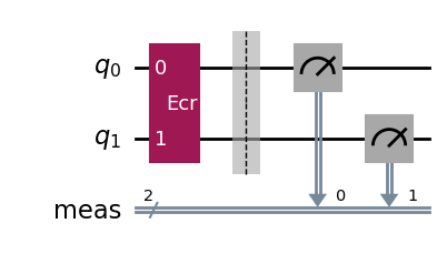
ECR gate
The ECR gate (Echoed Cross-Resonance gate) is the only two-qubit basis gate in the Eagle family of IBM QPUs (other families support the CZ or CX gate instead, see tables of gates). It is represented in the computational basis by the 4×4 matrix

Its action on the initial 2-qubit state is

The measurements of a noise-free ECR gate circuit are (0,1) with probability 1/2 and (1,1) with probability 1/2. The outcome (0,0) and (1,0) are not possible in the noise-free circuit.
qc = QuantumCircuit(2)
qc.ecr(0, 1)
dist, qc_isa = run_circuit(qc, num_shots=100_000)

qc_isa.draw(output="mpl", idle_wires=False, style="iqp")
print_results(dist)
Measurement counts: {'11': 49254, '01': 50325, '00': 239, '10': 182}
p(11): 0.4925  ± 0.0041
p(01): 0.5032  ± 0.0041
p(00): 0.0024  ± 0.0004
p(10): 0.0018  ± 0.0003
We observe a distribution of measured classical bits roughly agreeing with the expected ideal distribution, but the presence of quantum errors is revealed by the presence of a few (0,0) and (1, 0) outcomes.
The fidelity of the output state ρ is given by

As in the case of the SX-gate circuit, we cannot directly estimate the fidelity of the ρ state prepared by the ECR-gate circuit by measuring the output bits of the circuit, since it depends on off-diagonal terms in the ρ matrix.
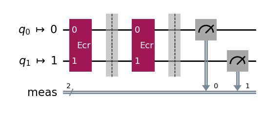
Instead we can follow the procedure described in the previous section and estimate a lower bound on F by considering the circuit with an added ECR⁻¹ gate. Since ECR⁻¹ = ECR, we consider a circuit with two ECR gates.
qc = QuantumCircuit(2)
qc.ecr(0, 1)
qc.barrier()  # Prevents circuit simplifications.
qc.ecr(0, 1)
dist, qc_isa = run_circuit(qc, num_shots=100_000)
qc_isa.draw(output="mpl", idle_wires=False, style="iqp")
print_results(dist)
Measurement counts: {'00': 99193, '01': 153, '10': 498, '11': 156}
p(00): 0.9919  ± 0.0007
p(01): 0.0015  ± 0.0003
p(10): 0.005  ± 0.0006
p(11): 0.0016  ± 0.0003
We find the estimated lower bound F > 0.9919 ± 0.0007 on the ρ state prepared by the ECR-gate circuit.
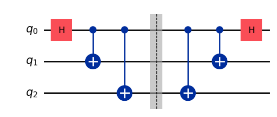
3-qubit state fidelity
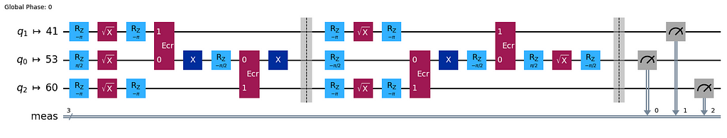
To close the loop, in our final example, let us compute a lower bound on the state fidelity of the 3-qubit state circuit which we considered first. Here again, we add the inverse operation to the circuit, bringing back the state to |0,0,0⟩ and measure the circuit outcomes.
qc = QuantumCircuit(3)
qc.h(0)
qc.cx(0, 1)
qc.cx(0, 2)
qc.barrier(). # Prevents circuit simplifications.
qc.cx(0, 2)
qc.cx(0, 1)
qc.h(0)
qc.draw('mpl')
dist, qc_isa = run_circuit(qc, num_shots=100_000)
qc_isa.draw(output="mpl", idle_wires=False, style="iqp")
print_results(dist)
Measurement counts: {'000': 95829, '001': 1771, '010': 606, '011': 503, '100': 948, '101': 148, '111': 105, '110': 90}
p(000): 0.9583  ± 0.0016
p(001): 0.0177  ± 0.0011
p(010): 0.0061  ± 0.0006
p(011): 0.005  ± 0.0006
p(100): 0.0095  ± 0.0008
p(101): 0.0015  ± 0.0003
p(111): 0.001  ± 0.0003
p(110): 0.0009  ± 0.0002
We find the fidelity lower bound F̃ = p’((0,0,0)) = 0.9583 ± 0.0016 for the 3-qubit state circuit.
Summary of results and discussion
Let us summarise our results in a table of fidelity lower bounds for the circuits we considered, using IBM QPUs.
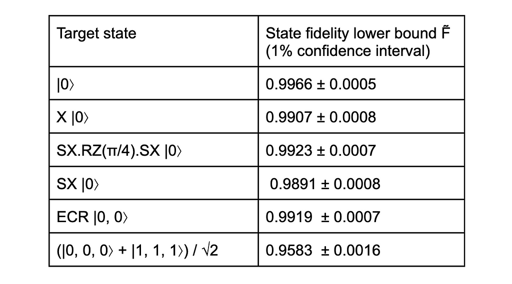
We find that the fidelity of states produced by circuits with a minimal number of basis gate is around 99%, which is not a small achievement. As we add more qubits and gates, the fidelity decreases, as we see with the 96% fidelity for the 3-qubit state, whose circuit has 13 basis gates. With more qubits and circuit depth, the fidelity would decrease further, to the point that the quantum computation would be completely unreliable. Nevertheless, these results look quite encouraging for the future of quantum computing.
It is likely that more accurate and rigorous methods exist to evaluate the fidelity of the state produced by a quantum circuit, giving more robust bounds. We are just not aware of them. The main point was to provide hands-on examples of Qiskit circuit manipulations for beginners and to get approximate quantum noise estimates.
While we have run a number of circuits to estimate quantum noise, we have only scratched the surface of the topic. There are many ways to go further, but one important idea to make progress is to make assumptions on the form of the quantum noise, namely to develop a model for a quantum channel representing the action of the noise on a state. This would typically involve a separation between “coherent” noise, preserving the purity of the state, which can be described with a unitary operation, and “incoherent” noise, representing interactions with the environment. The Qiskit Summer School lecture on the topic provides a gentle introduction to these ideas.
Finally, here are a few reviews related to quantum computing, if you want to learn more on this topic. [1] is an introduction to quantum algorithms. [2] is a review of quantum mitigation techniques for near-term quantum devices. [3] is an introduction to quantum error correction theory. [4] is a review of quantum computing ideas and physical realisation of quantum processors in 2022, aimed at a non-scientific audience.
Thanks for getting to the end of this blogpost. I hope you had some fun and learned a thing or two.
Unless otherwise noted, all images are by the author
[1] Blekos, Kostas and Brand, Dean and Ceschini, Andrea and Chou, Chiao-Hui and Li, Rui-Hao and Pandya, Komal and Summer, Alessandro, Quantum Algorithm Implementations for Beginners (2023), Physics Reports Volume 1068, 2 June 2024.
[2] Cai, Zhenyu and Babbush, Ryan and Benjamin, Simon C. and Endo, Suguru and Huggins, William J. and Li, Ying and McClean, Jarrod R. and O’Brien, Thomas E., Quantum error mitigation (2023), Reviews of Modern Physics 95, 045005.
[3] J. Roffe, Quantum error correction: an introductory guide (2019), Contemporary Physics, Oct 2019.
[3] A. K. Fedorov, N. Gisin, S. M. Beloussov and A. I. Lvovsky, Quantum computing at the quantum advantage threshold: a down-to-business review (2022).
Measuring Quantum Noise in IBM Quantum Computers was originally published in Towards Data Science on Medium, where people are continuing the conversation by highlighting and responding to this story.
Originally appeared here:
Measuring Quantum Noise in IBM Quantum Computers
Go Here to Read this Fast! Measuring Quantum Noise in IBM Quantum Computers